LoopVQ:面向循环 Transformer 的亚 1-bit KV 缓存量化 LoopVQ: Sub 1-bit KV Cache Quantization for Looped Transformers
跨循环步联合向量量化 KV 缓存并微调码本,0.5/0.25 bit 下接近 BF16 精度
前置知识
KV 缓存 (KV cache)
自回归解码时,为避免每生成一个 token 就重算整段序列,推理引擎会把每个 token 在每层的 key 和 value 向量缓存下来。标准 Transformer 每个 token、每层存一份 K/V,缓存大小随上下文长度线性增长,是长上下文与大批量服务的主要显存瓶颈。
本文的全部工作都围绕 KV 缓存的压缩展开,论文的核心观察(循环步间冗余)就是针对循环模型中每个循环步各自一份缓存的结构。
循环 Transformer (Looped LM)
用同一组层(参数 $\theta$)反复应用 $T$ 次的架构:循环步 $t$ 把上一步的隐状态 $h^{(t-1)}$ 再喂进同一组层得到 $h^{(t)}$,输出分布取自最后一步。Ouro 用 24/48 层的块循环 4 次,Huginn 把 4 层核心块循环 32 次。参数量大幅缩减,性能可匹配数倍于自身的非循环模型。
循环架构是本文的适用对象:它省参数但每个循环步各存一份 KV,缓存反而比同规模标准模型大 $T$ 倍,成为其部署瓶颈。
向量量化 (Vector Quantization) 与码本
把 $D$ 维缓存向量切成 $G$ 个连续信道的子向量,对每类子向量用 k-means 学一个含 $K=2^b$ 个条目的码本 $\mathcal{B}$,缓存中只存最近邻条目的 8-bit 索引 $a(z)=\arg\min_r\|z-e_r\|_2^2$,每元素成本为 $b/G$ bit。码本通常按(层、头、信道组)离线校准。
LoopVQ 属于 VQ 一族(与 CQ、TaSQ 同类),理解子向量、码本、索引、b/G bit 这些概念是看懂其『一个索引服务多个循环步』设计的前提。
RoPE 旋转位置编码
RoPE 把相对位置信息以复数旋转的方式注入 query 和 key,同一个 key 在不同位置会被旋转不同角度。因此 KV 缓存量化方法普遍在施加 RoPE 之前量化 key(pre-RoPE),注意力计算时对重建出的 key 再按其位置施加 RoPE。
LoopVQ 及所有基线都在 pre-RoPE 上量化,注意力内核必须对每条重建的 key 做 RoPE,这直接决定了其 CUDA/Triton 内核的设计(预计算余弦正弦表等)。
Fisher 加权 k-means
朴素 k-means 对所有子向量一视同仁,而不同向量对模型输出的影响不同。Fisher 加权版本给每个子向量乘权重 $\omega_n=\|\partial L/\partial z_n\|_2^2$(对下一 token 损失的梯度范数平方,即经验 Fisher 信息对角和),误差落在敏感向量上罚得更重。这是 CQ 等先前 KV VQ 方法使用的校准目标。
LoopVQ 用它初始化码本,但论文证明它无法表达跨循环步误差交互与步间敏感度差,因此必须换成输出 KL 微调——理解这一点才能看懂方法第 4.2 节的动机。
KL 散度与知识蒸馏式微调
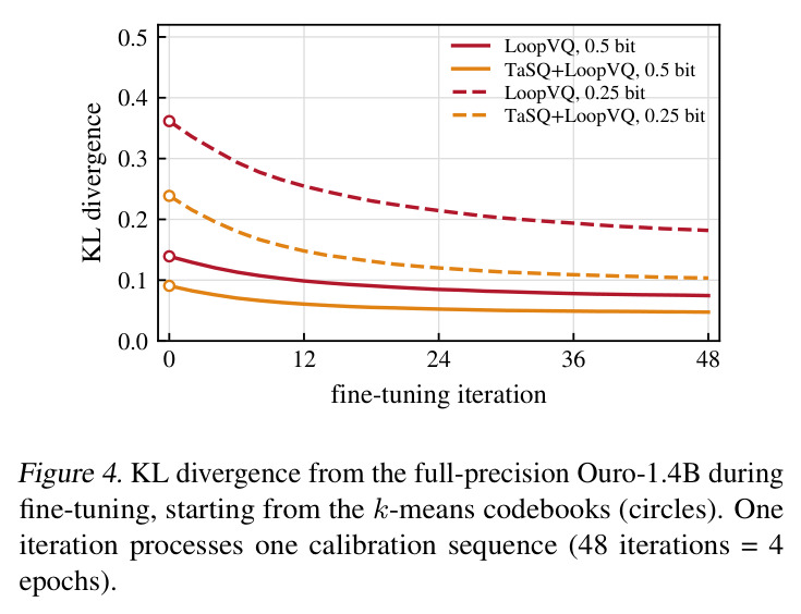
KL 散度 $\mathrm{KL}(p\|q)=\sum_i p_i\log(p_i/q_i)$ 衡量两个分布的差异。知识蒸馏用教师模型的输出分布监督学生模型。LoopVQ 把全精度模型输出 $p_j$ 当教师、量化模型输出 $q_j(\mathcal{B})$ 当学生,冻结权重只调码本,最小化 $J(\mathcal{B})=\mathbb{E}_s[\frac{1}{N}\sum_j \mathrm{KL}(p_j\|q_j)]$。
这是 LoopVQ 码本微调的目标函数(式 6),也是它显著超越加权 k-means 的关键:直接匹配模型端到端输出而非逐向量重建误差。
SGLang 与 Flash-Decoding 式注意力
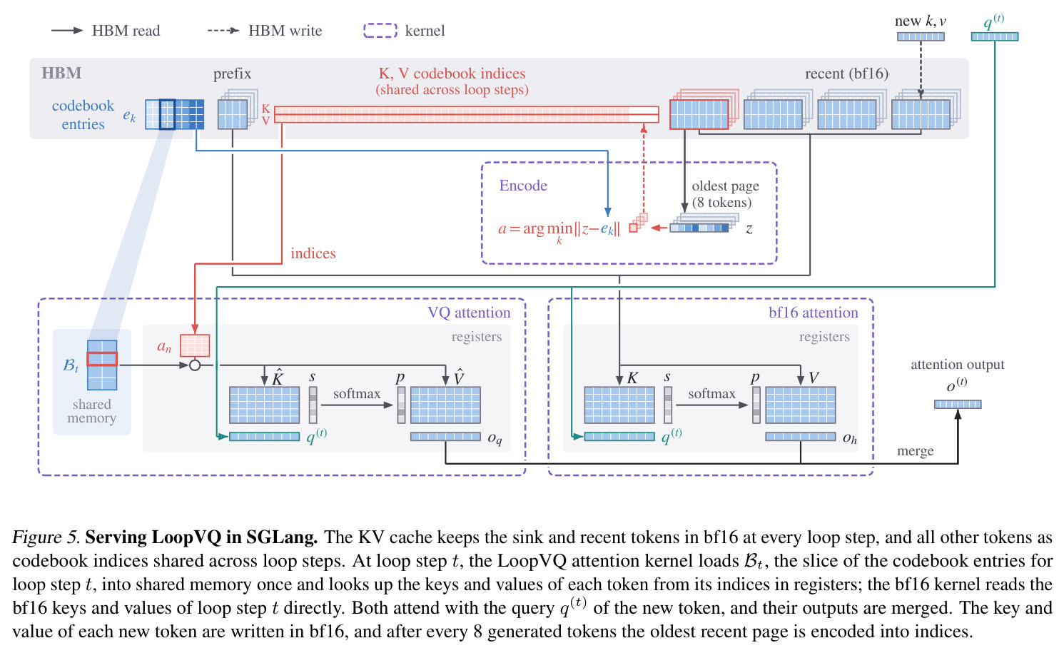
SGLang 是主流 LLM 推理服务框架。Flash-Decoding 把解码注意力的 KV 序列切成多个 split,由不同线程块并行计算部分 softmax 结果,再用 logsumexp 精确合并。LoopVQ 的量化注意力内核复用这一方案,并用 shared memory 缓存码本切片、按索引查表重建 K/V。
论文第 4.3 节和所有延迟/吞吐结果都基于其 SGLang 实现,不了解这套 serving 机制就看不懂缓存分页、sink/recent 窗口等工程细节。
研究动机
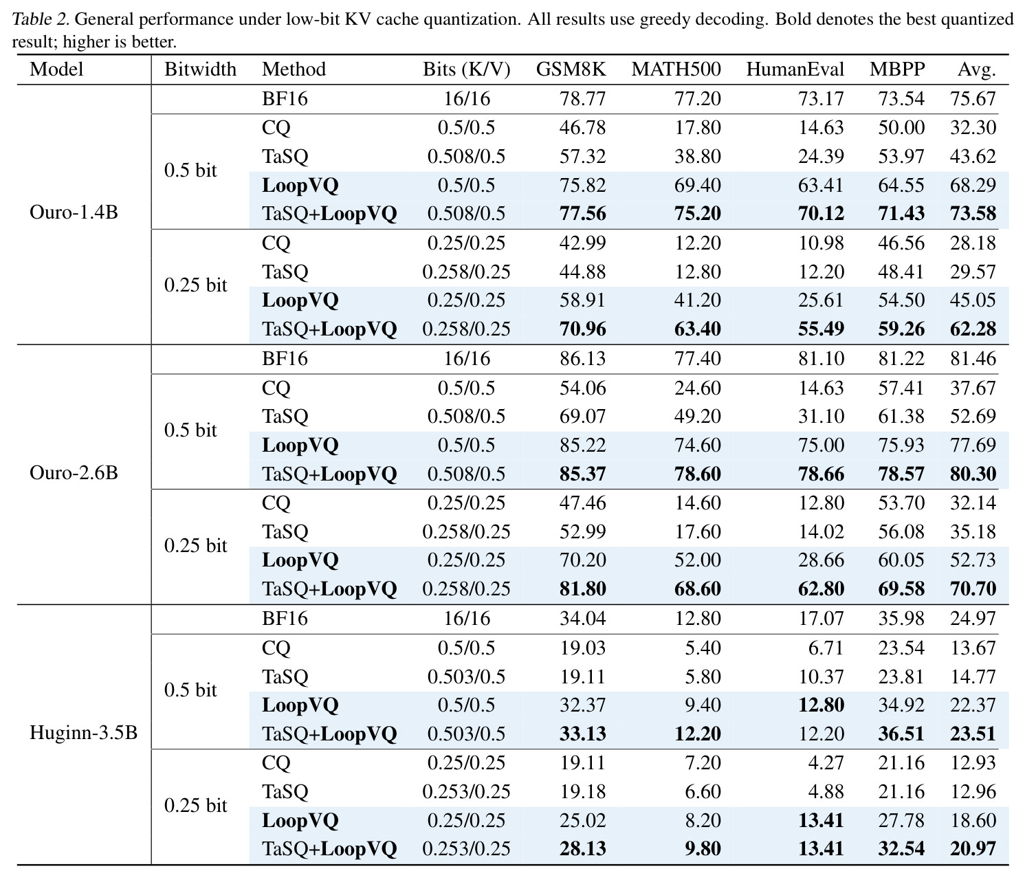
循环 Transformer 用参数复用换来了极小的权重显存(Ouro-1.4B 性能可比肩数倍于它的非循环模型),但这个效率完全没有延伸到 KV 缓存:虽然 $T$ 个循环步共享同一组权重,每个循环步仍各自存一套 key/value,缓存随循环步数线性增长。论文图 1a 显示,Ouro-1.4B 每 token 的 KV 缓存(bf16)是 Llama-3.1-8B 的 6 倍,在中等上下文长度下缓存就已经超过模型权重本身,这直接限制了可服务的批大小与上下文长度。已有的 KV 量化方法(CQ、TaSQ 等)是为非循环模型设计的:它们把同一层 $T$ 个循环步的缓存当作互不相关的独立缓存,逐循环步分别学习码本,完全无法利用循环结构带来的冗余。结果是亚 1 bit 区域精度崩塌:在 Ouro-1.4B 的 GSM8K/MATH500/HumanEval/MBPP 四任务平均上,BF16 为 75.67,0.5 bit 下 CQ 只有 32.30、TaSQ 只有 43.62;在长思维链推理任务上退化更严重(CQ 平均只剩 15.65,BF16 为 56.43),大量推理序列还会因误差提前终止或撞到生成长度上限。
本文的目标是本文的目标是:在不丢弃任何 token、不修改模型结构、不重训权重的前提下,把循环语言模型的 KV 缓存压缩到每元素 0.5 bit 甚至 0.25 bit(低于现有循环模型 KV 量化方法 FlashLoop/ResidualQuant 的 2-4 bit 区间),同时在通用基准(GSM8K、MATH500、HumanEval、MBPP)、长思维链推理(AIME、GPQA-Diamond、HumanEval+、MBPP+)和长上下文检索(RULER NIAH、LongBench)三类任务上尽可能保留 BF16 精度;并把方法实装进 SGLang 推理引擎,让量化真正转化为解码延迟降低和服务吞吐提升,而不是停留在离线精度数字上。
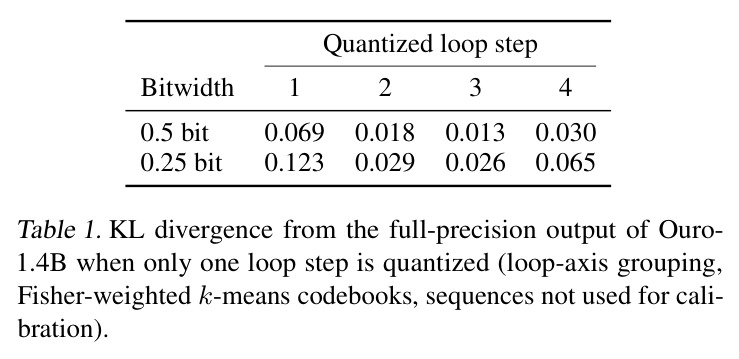
与已有工作不同的是,本文的独特切入是把『循环步』当作向量量化的一个全新分组轴。作者先用两个实证观察支撑这个角度:其一,同一 token 在各循环步的 key/value 高度相似——相邻循环步间平均相关系数从首两步的 0.69 升到末两步的 0.94,一个 key 信道与相邻循环步同一信道的平均相关 $|r|=0.85$,而与同组其他信道仅 0.16,value 上差距更大——说明把多个循环步的信道编进同一个子向量能大幅降低重建误差;其二,各循环步对量化的敏感度差约 5 倍(只量化单个循环步时,输出 KL 从第一步的 0.069 到第三步的 0.013)。已有的循环模型量化工作要么针对共享块的权重/激活(LoopQ、LoopQuant、Loopy),要么对 KV 做每元素至少 1 bit 的标量量化(FlashLoop、ResidualQuant),没有人利用循环轴冗余在亚 1 bit 区间做 KV 向量量化。
核心方法
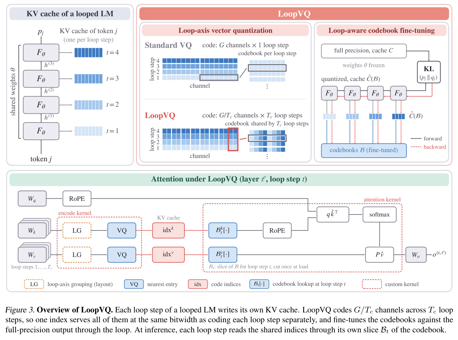
直觉上,循环模型的 $T$ 个循环步缓存是由同一组投影权重从同一个 token 的隐状态逐步计算出来的,彼此高度相似,因此可以让多个循环步『共用一个索引』:把 $T_c$ 个循环步各取 $G/T_c$ 个信道拼成一个耦合子向量,用一个 8-bit 码字索引同时重建它们,位宽与逐循环步量化完全相同、零额外开销。但误差在不同循环步上的危害不同(早期循环步的误差会经递归传播污染所有后续步),逐向量的 k-means 目标无法表达这一点,所以校准分两阶段:先用 Fisher 加权 k-means 初始化码本,再冻结模型权重、以全精度模型输出分布为教师做端到端 KL 微调。工程上,LoopVQ 实装进 SGLang:少量 sink/recent token 保 bf16,其余 token 存跨循环步共享的码本索引,解码时每个循环步通过码本的自己的切片查表重建 K/V 并施加 RoPE,用 Flash-Decoding 式 split 并行与 logsumexp 合并。整体由三部分组成:loop 轴向量量化(4.1 节)、loop 感知码本微调(4.2 节)、系统实现(4.3 节)。
核心创新有两点,都与已有方法有本质区别。第一,loop 轴分组:现有 KV VQ 方法(CQ 沿信道分组、TaSQ 沿信道轴变换)只在信道轴上做文章,且逐循环步独立编码;LoopVQ 让一个码字覆盖 $c=G/T_c$ 个信道 × $T_c$ 个连续循环步,同一索引服务 $T_c$ 个循环步,位宽保持 $b/G$ bit/元素不变——循环轴是免费的额外压缩自由度,且与信道轴方法正交、可组合(TaSQ+LoopVQ)。第二,loop 感知码本微调:加权 k-means 的目标是每个耦合向量误差的独立加权和,而论文在附录 A.1 中证明,输出 KL 目标的二阶近似 $J\approx\frac{1}{2}\mathbb{E}_s[\delta^\top F\delta]$ 中的 Fisher 交叉块 $F_{nn'}$ 连接了同一 token 在不同循环步、不同层的码字误差(早期步误差会传播并与后续步误差叠加),任何加权 k-means 都只能匹配对角块 $F_{nn}$、必然丢掉交叉项,因此必须直接对输出 KL(式 6)做端到端微调,且每次迭代重算最近邻分配,保证码本始终在推理时实际使用的编码器下训练。
方法步骤详情
方法可拆成五步。第一步,loop 轴分组:把 $T$ 个循环步划成大小为 $T_c$ 的连续块($T_c$ 须同时整除 $T$ 和 $G$),对层 $\ell$、头 $h$、信道组 $g$,token $j$ 的耦合向量第 $iT_c+m$ 个坐标取自循环步 $\beta T_c+m+1$ 的信道 $g_{c+i}$($i<c$,$m<T_c$,$c=G/T_c$),即一个码字横跨 $c$ 个信道 × $T_c$ 个循环步;key 在 RoPE 之前量化。第二步,初始化:用 Fisher 加权 k-means(式 3)初始化码本 $\mathcal{B}_{\beta,\ell,h,g}$,权重 $\omega_n$ 把所覆盖 $T_c$ 个循环步的梯度平方求和。第三步,微调:冻结权重,最小化 $J(\mathcal{B})=\mathbb{E}_s[\frac{1}{N}\sum_j \mathrm{KL}(p_j\|q_j(\mathcal{B}))]$,其中 $q_j$ 是所有 $T$ 个循环步都 attend 到重建缓存时的输出;分配由 arg min 得到、无需直推估计,码本条目经链式法则获精确梯度(附录 A.2);每迭代处理一条校准序列(Adam,学习率 $10^{-3}$,4 个 epoch,12 条训练、4 条按最低 KL 选优),输入为 16 条 2048-token 的 GPQA 序列;代价极低——RTX 6000 Ada 上 Ouro-1.4B 的 k-means 加微调共 6.1+2.3 分钟。第四步,缓存布局与编码:每请求前 8 个 sink 与最近 64(长上下文 256)个 token 保 bf16,其余按 8-token 页存索引;耦合向量要等块内最后一个循环步算完才能编码,prefill 时在 tensor core 上以矩阵乘批量完成,解码每生成 8 个 token 把窗口最旧页编码一次。第五步,注意力内核:量化内核把本循环步的码本切片 $\mathcal{B}_t$(加载时切割一次)载入 shared memory,按 $D/c$ 个索引查表重建 key、施加 RoPE、计算注意力分数;量化页与 bf16 页分别用两个内核 attend,部分结果按 Flash-Decoding 方式用 logsumexp 精确合并;批处理时两个请求共享一个线程块与 RoPE 表、码本载入,使 batch 64、6K 上下文的解码注意力时间再降 37%/48%。
技术新颖性
技术新颖性体现在四个层面。问题层面:这是首个面向循环语言模型的亚 1-bit KV 缓存向量量化方法,此前循环模型的 KV 压缩(FlashLoop、ResidualQuant)只有 2-4 bit 标量量化,物理上到不了 0.25-0.5 bit 区间。观察层面:论文给出了可复用的实证结论——循环轴是高度冗长的压缩轴(loop 轴分组让普通 k-means 在 0.5 bit 的重建误差在 Ouro-1.4B 上约减半),且循环步敏感度差约 5 倍(KL 0.069/0.018/0.013/0.030 @0.5bit),这两个观察独立于具体量化算法。理论层面:附录 A.1 用 Fisher 矩阵的分块分解严格证明了『任何加权 k-means 目标都无法表达输出目标』——交叉块 $F_{nn'}$ 承载跨循环步误差交互,加权 k-means 只能对角化——为端到端码本微调提供了原则性依据,而非经验性选择。系统层面:跨循环步共享索引带来非平凡的内核设计(每 $T_c$ 步一行索引的存储布局、按步切割的码本切片、RoPE 预计算表跨请求共享、双请求共线程块),并与信道轴方法 TaSQ 组合时联合优化了信道置换 $P$ 使分组同时覆盖 RoPE 配对坐标与跨步相关信道(附录 B)。
实验结果
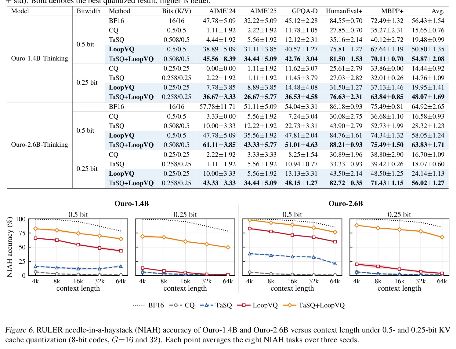
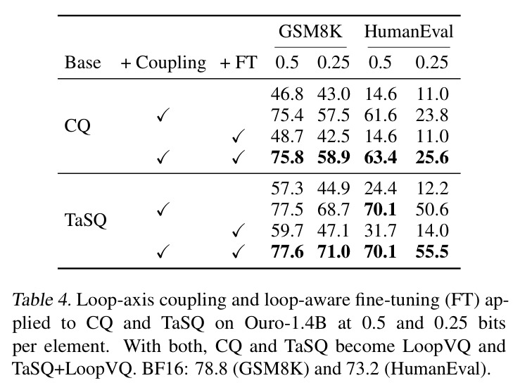
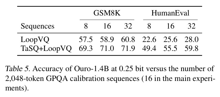
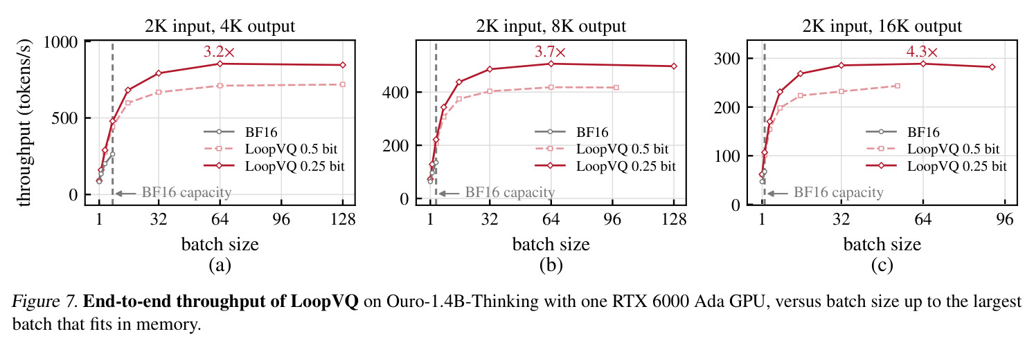
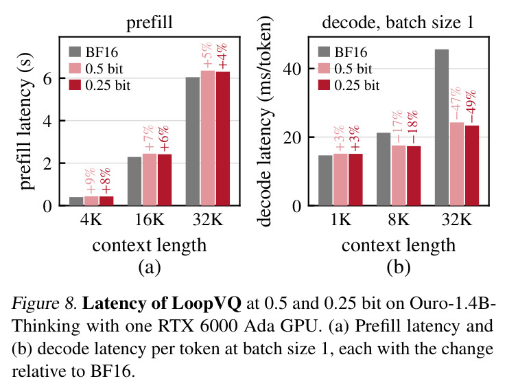
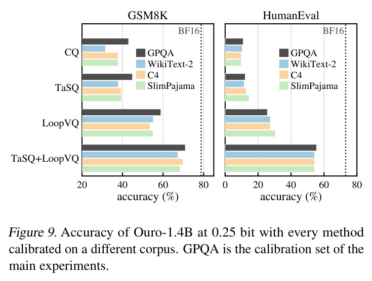
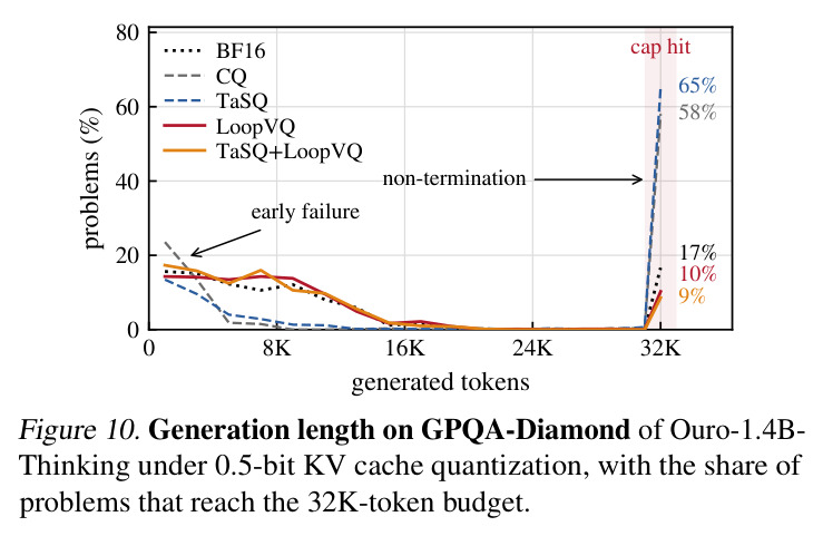
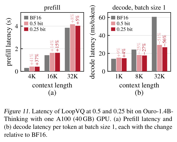
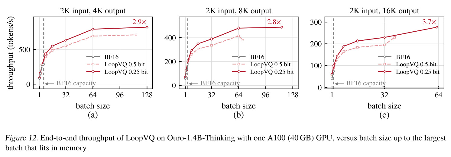
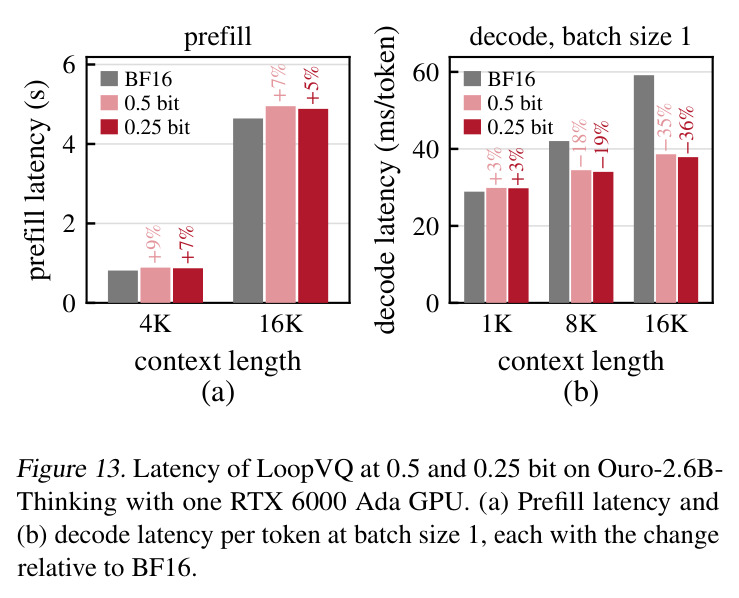
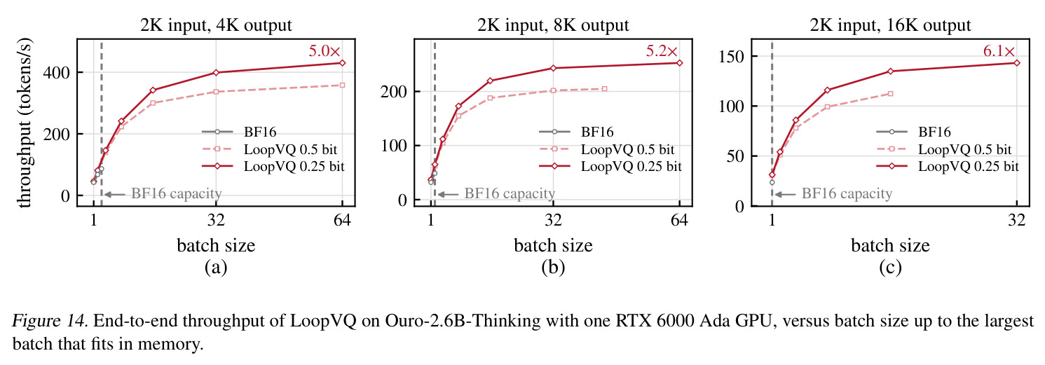
通用基准(Table 2,贪心解码):Ouro-1.4B 四任务平均 BF16 为 75.67,0.5 bit 下 CQ 只有 32.30、TaSQ 43.62,而 LoopVQ 达 68.29、TaSQ+LoopVQ 达 73.58(GSM8K 77.56 几乎追平 BF16 的 78.77);0.25 bit 下 TaSQ+LoopVQ 平均 62.28,基线只有 28-30。Ouro-2.6B 平均 BF16 81.46,0.5 bit TaSQ+LoopVQ 80.30(近乎无损),0.25 bit 仍达 70.70。结构迥异的 Huginn-3.5B(4 层核心块循环 32 次)结论一致:BF16 24.97,0.5 bit TaSQ+LoopVQ 23.51,基线只有 13-15。长思维链推理(Table 3,3 采样种子):基线崩塌最严重——Ouro-1.4B-Thinking 五任务平均 BF16 56.43,CQ@0.5bit 仅 15.65、AIME'24 仅 1.11,而 LoopVQ 保住 50.80、TaSQ+LoopVQ 54.87;0.25 bit 下 TaSQ+LoopVQ 48.07(AIME'24 45.56 vs BF16 47.78)。Ouro-2.6B-Thinking 平均 BF16 64.92,TaSQ+LoopVQ 为 63.83/56.02,全面领先。长上下文(Figure 6、Table 6):RULER 全部 8 项 NIAH(4K-64K)中基线在所有长度都远低于 BF16,LoopVQ@0.5bit 能取回大部分 needle,TaSQ+LoopVQ 在每个长度与位宽都最高;LongBench 16 个英文任务上 TaSQ+LoopVQ@0.5bit 达 29.04,与 BF16 的 29.67 相差不到 1.5 点。系统效率(Figure 7/8,RTX 6000 Ada):batch 1 解码在 32K 上下文延迟较 BF16 降 47%/49%,prefill 因编码慢 3%-9%;缓存读取字节少 8×/16× 使 BF16 只能容纳几个请求而 LoopVQ 可服务数十到上百并发,峰值吞吐达 BF16 的 3.2×-4.3×(Ouro-1.4B)与 5.0×-6.1×(Ouro-2.6B);batch 16、32K 时注意力耗时从 1.87 ms/token 降到 0.63/0.54 ms,编码仅占解码 <1%、prefill 5-7%。消融(Table 4):耦合贡献绝大部分增益(CQ GSM8K 46.8→75.4),微调再补(→75.8,HumanEval 57.5→61.6),组合在每个设置最优或并列最优。稳健性(Figure 9、Table 5):换校准语料 CQ 波动最多 11 点,TaSQ+LoopVQ ≤4 点且始终最好;校准序列 8→32 条持续涨分。推理稳定性(Figure 10、附录 D.4):CQ/TaSQ 大量问题撞 32K 预算或提前终止(Ouro-2.6B-Thinking@0.25bit 的 CQ 有 59% 生成在 2K 内结束,BF16 为 22%),LoopVQ@0.5bit 保持 BF16 的长度分布,吞吐增益能兑现为答题时间缩短。
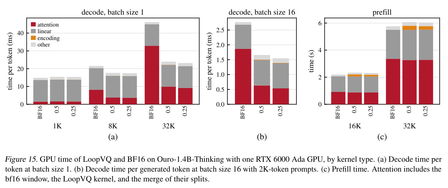
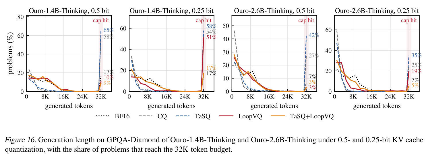
查看结构化数据
| 任务 | 指标 | 本文 | 基线 | 提升 |
|---|---|---|---|---|
| 通用四基准平均(Ouro-1.4B,0.5 bit) | 平均准确率 (%) | TaSQ+LoopVQ 73.58(LoopVQ 单独 68.29) | BF16 75.67;最强基线 TaSQ 43.62 | 较最强基线 +29.96 点,距 BF16 仅 -2.09 点 |
| 通用四基准平均(Ouro-1.4B,0.25 bit) | 平均准确率 (%) | TaSQ+LoopVQ 62.28 | CQ 28.18 / TaSQ 29.57 | +32.71 至 +34.10 点 |
| 长 CoT 推理五任务平均(Ouro-1.4B-Thinking,0.25 bit) | 平均准确率 (%) | TaSQ+LoopVQ 48.07(LoopVQ 19.95) | BF16 56.43;CQ 14.44 / TaSQ 14.76 | 较基线 +33.31 点以上,保留 BF16 的 85% |
| AIME'24(Ouro-1.4B-Thinking,0.5 bit) | 准确率 (%) | TaSQ+LoopVQ 45.56 | BF16 47.78;CQ 1.11 | 仅比 BF16 低 2.22 点,基线崩溃至 1.11 |
| RULER NIAH(Ouro-1.4B/2.6B,4K-64K 上下文) | 8 项任务平均准确率 (%) | TaSQ+LoopVQ 在每个长度、每个位宽上都最高 | CQ / TaSQ 在所有长度远低于 BF16 | 0.5 bit 下 LoopVQ 即可取回大部分 needle |
| LongBench 16 个英文任务(Ouro-1.4B,0.5 bit) | 各任务官方指标平均 | TaSQ+LoopVQ 29.04 | BF16 29.67;CQ 21.37 / TaSQ 23.00 | 与 BF16 相差 0.63 点,领先基线 6 点以上 |
| 解码延迟(Ouro-1.4B-Thinking,32K 上下文,batch 1) | ms/token 相对 BF16 变化 | 0.5 bit -47%,0.25 bit -49% | BF16 | 长上下文解码延迟约减半 |
| 峰值服务吞吐(Ouro-2.6B-Thinking,RTX 6000 Ada) | tokens/s(2K 输入,4K-16K 输出) | 最高达 BF16 的 6.1× | BF16(显存仅容 1-3 个长请求) | 5.0×-6.1×;Ouro-1.4B 上为 3.2×-4.3× |
局限与改进
作者在 Limitations 节明确承认两点:其一,效率评估只与 BF16 serving 对比,没有与其他量化方法对比,因为每种方法的内核都为其缓存格式单独优化,很难保证可比的优化水平,他们选择与 SGLang 已高度优化的 BF16 对比以避免偏向自己;其二,精度上没有与循环模型专用的 KV 量化方法 FlashLoop、ResidualQuant 对比,理由是它们是 2-4 bit 的标量量化、不提供亚 1 bit 配置,属于不同赛道。我自己的观察还有几条:0.25 bit 虽然仍大幅领先基线,但绝对精度损失不小(Ouro-1.4B 通用平均 62.28 vs 75.67,HumanEval 55.49 vs 73.17,Huginn-3.5B 通用平均只有 20.97 vs 24.97),亚 1 bit 并非无损;方法需要逐模型校准,校准语料的选择虽有稳健性实验支撑但只用 3 个英文语料验证;TaSQ+LoopVQ 的实际 key 位宽略高于名义值(0.508/0.258,另有 fp16 尺度因子约 0.008 bit/元素);实验只覆盖 Ouro(T=4)与 Huginn(核心块循环 32 次但仅 4 层)两族 1.4B-3.5B 的密集多头注意力模型,没有 GQA/MQA、更大规模或多模态的结果;bf16 sink/recent 窗口大小与 8-token 页大小都是手工设定的超参数,未做敏感性分析。
独立分析的弱点
第一,耦合分组与实测敏感度差异内在矛盾:Table 1 证明各循环步敏感度差约 5 倍(第一步最 harmful、第三步最不敏感),但一个码字内 $T_c$ 个循环步被强制等精度,微调只能部分弥补。改进方向是混合精度耦合——对首个循环步保留更小的 $c$ 或独立码本,或按 Fisher 权重非均匀分配码本条目数。第二,块边界固定为连续 $T_c$ 步,未利用『相关性随循环步深入而增强(0.69→0.94)、首步最敏感』的结构信息,自适应分组(如把首步与末步配对、或按层/头动态选 $T_c$)值得探索。第三,prefill 编码带来最高 +9% 的延迟开销,论文只展示了 2K 输入的长输出场景,对长输入短输出(如长文档摘要、RAG 首响)这类 prefill 密集型负载是否划算没有数据支撑,应补充该场景评测或设计异步/摊销编码。第四,校准依赖 16 条 2048-token 的 GPQA 序列,跨语料实验只有三个英文语料,代码、多语言、多轮对话等分布外的稳健性未知;可以引入按任务域检索校准样本或在线校准。第五,0.25 bit 下与 TaSQ 组合仍有明显掉点(HumanEval 55.49 vs 73.17),说明代码生成对缓存误差更敏感,可针对任务类型自适应选择位宽。第六,效率只对比 BF16 的论证虽然合理,但缺少与 2-4 bit 标量方案(FlashLoop/ResidualQuant)在『精度-位宽』全曲线上的对比,读者无法判断 0.25 bit LoopVQ 是否真的优于 2 bit 标量量化在相同显存预算下的表现,这是实验设计上最值得补的一块。
未来方向
作者明确提出的延伸是把校准集扩大(校准只需分钟级,Table 5 显示 8→32 条仍有稳定收益,可以更低成本换更高精度)。基于本文成果可以延伸的方向:其一,与共享块权重/激活量化(LoopQ、LoopQuant、Loopy)协同,把循环模型压成全低 bit 推理栈,权重共享结构使循环模型的权重量化与 KV 量化天然正交;其二,把『loop 轴作为量化分组轴』的思想推广到更一般的循环深度/latent 推理架构(如 recurrent-depth 模型、CoT-in-latent 类模型),只要存在同一参数的多次应用就存在轴间冗余;其三,按敏感度自适应的混合精度方案——不同循环步、不同层、不同头使用不同 $c$ 或码本大小 $K$;其四,把附录 B 的启发式 covariance 信道置换升级为与循环耦合联合优化的可学习置换;其五,将输出 KL 码本微调范式迁移到其他缓存压缩场景,如跨层 KV 共享、KV 驱逐恢复(作者组里的 KV-Rescue);其六,与推测解码、稀疏注意力、GQA 的组合实验;其七,服务侧可做量化页的在线重校准以跟踪分布漂移,以及在张量并行/多卡 serving 下的扩展。最后,把『量化误差改变生成长度进而影响真实时延』的评估方法论(Figure 10、附录 D.4)推广为 KV 压缩的标准评测协议,本身就是一个有价值的后续工作。
复现评估
复现条件相当好。代码已开源(GitHub: mscheong01/LoopVQ),模型全部公开(Ouro-1.4B/2.6B 及其 Thinking 变体来自 Zhu et al. 2025,Huginn-3.5B 来自 Geiping et al. 2026),评测基准都是标准公开数据集(GSM8K 3-shot CoT、MATH500、HumanEval/MBPP 及 + 版本、AIME'24/'25、GPQA-Diamond、RULER 8 项 NIAH、LongBench 16 个英文任务),校准数据为 16 条 2048-token 的 GPQA main 序列(排除与评测重叠的 Diamond 子集)。校准成本极低且论文给出了具体数字:单张 RTX 6000 Ada 上 k-means 加微调,Ouro-1.4B 共 6.1+2.3 分钟、Ouro-2.6B 共 14.3+5.9 分钟(A100 上 5.5+2.0 / 11.2+4.6 分钟),不需要大规模算力。算法部分的复现难度为中等偏低:有码本初始化、微调目标(式 6)、梯度计算(附录 A.2)的完整描述。系统部分的复现难度较高:需要在 SGLang 中实现跨循环步共享索引的缓存布局、pre-RoPE 量化注意力 Triton 内核(Algorithm 1,含 RoPE 预计算表、shared memory 码本切片、双请求共线程块等优化),延迟/吞吐数字依赖同代 GPU(RTX 6000 Ada 48GB,A100 结果在附录提供),普通用户照论文数字复现性能需要相当的内核工程能力,但精度结果应容易对齐。
论文图表
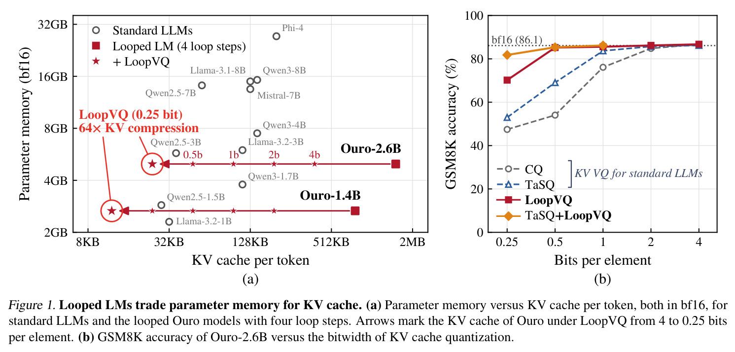
双面板动机图。(a) 以对数坐标对比标准 LLM(Llama、Qwen、Mistral 等)与循环 Ouro 模型的参数显存和每 token KV 缓存:Ouro 参数小但 KV 缓存反而比大得多的标准模型更高(Ouro-1.4B 的每 token KV 约为 Llama-3.1-8B 的 6 倍),箭头标出 LoopVQ 把 Ouro 的 KV 从 4 压到 0.25 bit/元素后的位置(64× KV 压缩,bf16 16GB 降到 2GB 以下)。(b) Ouro-2.6B 的 GSM8K 准确率随 KV 量化位宽的变化,显示为标准 LLM 设计的 KV VQ(CQ、TaSQ)在低位宽下精度快速下降,而 LoopVQ/TaSQ+LoopVQ 曲线保持高位。
一图道尽论文的动机与主张:循环模型省参数却爆 KV 缓存,现有方法在亚 1 bit 失效,而 LoopVQ 能在 0.25 bit 保住大部分精度。
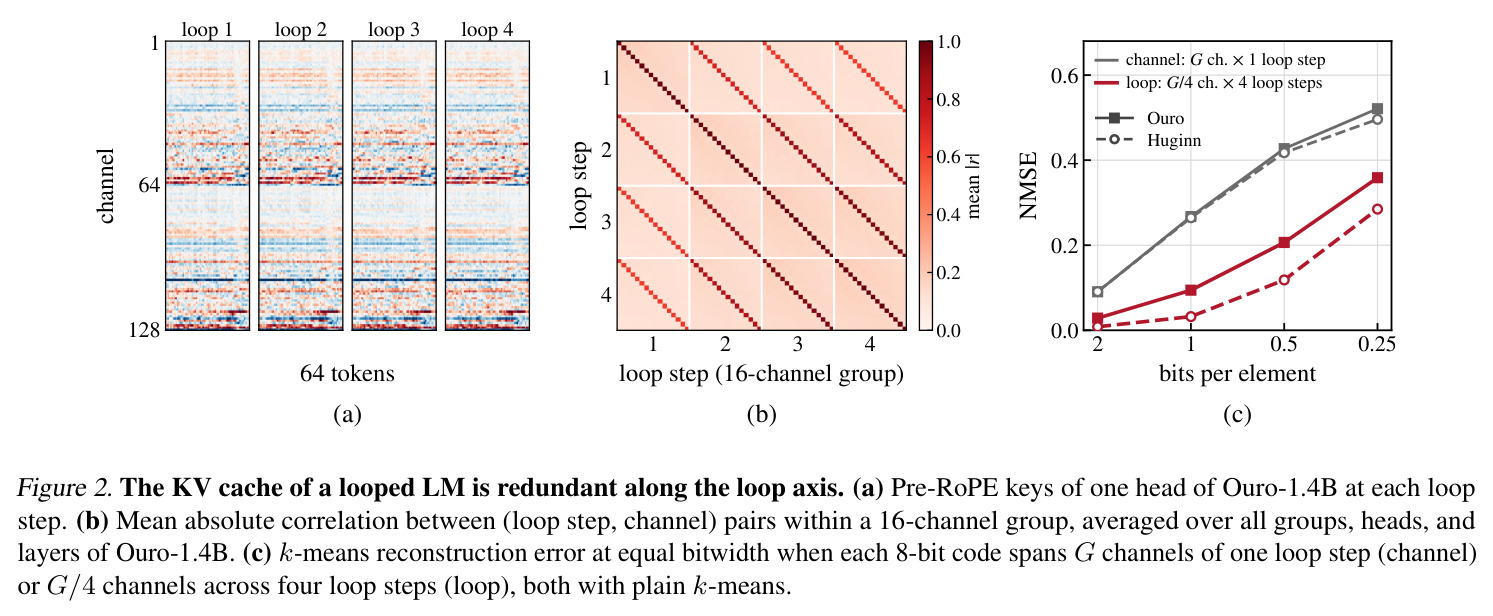
三面板核心观察图。(a) 一个头的 pre-RoPE key 在 4 个循环步上的热图,信道模式几乎相同,直观展示跨步相似性;(b) 16 信道组内(循环步,信道)坐标对之间的平均绝对相关:同一信道在相邻循环步之间相关高达 0.85(步间平均相关 0.69→0.94),而组内不同信道仅 0.16;(c) 在相同位宽与码本数下,比较『G 信道 × 1 循环步』(channel 分组)与『G/4 信道 × 4 循环步』(loop 分组)的 k-means 重建误差,后者在 Ouro-1.4B@0.5bit 上约减半,且在两个模型所有位宽(2/1/0.5/0.25 bit)上都显著更低。
这是全文最重要的实证依据:证明循环轴是高度冗余且与信道轴不同的量化分组轴,是 LoopVQ 设计合理性的根基。
校准序列数从 8 条增加到 16、32 条时 Ouro-1.4B@0.25bit 的准确率:LoopVQ GSM8K 57.5→58.9→60.8、HumanEval 22.6→25.6→28.0;TaSQ+LoopVQ GSM8K 69.3→71.0→71.9、HumanEval 49.4→55.5→59.8。即使最小 8 条也远超基线。
给出校准成本的定量指引:精度随校准集单调提升且校准本身只需分钟级,用户可按需加大校准规模。
LongBench 16 个英文任务(单文档 QA、多文档 QA、摘要、few-shot、合成、代码六大类)逐任务结果:CQ/TaSQ 平均比 BF16 低 7-13 点;LoopVQ 在所有设置下平均领先两个基线;TaSQ+LoopVQ@0.5bit 达 29.04(BF16 29.67,相差不到 1.5 点),Ouro-2.6B 上 35.69(BF16 37.18)。
在 RULER 之外用更真实多样的长文本任务验证泛化性,补全长上下文能力的证据链。
Figure 10 的扩展:两个 Thinking 模型 × 两个位宽共四个设置下的 GPQA-Diamond 生成长度分布。CQ 与 TaSQ 在所有设置都有大量问题耗尽生成预算(Ouro-1.4B-Thinking@0.25bit CQ 撞顶 65%)或提前终止;TaSQ+LoopVQ 在全部四个设置都保持 BF16 的长度分布,LoopVQ@0.5bit 亦然。
系统性地证明 LoopVQ 不会像基线那样把误差转化为更多推理 token,吞吐优势能兑现为实际答题提速。