← 返回 2026-10-19

DAGFormer：面向Transformer跨层连接的全局拓扑预测 DAGFormer: Global Topology Prediction for Transformer Cross-Layer Connections

Xiaocong Yang, Yuren Hao, ChengXiang Zhai 📅 2026-10-14 👍 8 2026-11-11 18:30

Transformer架构动态跨层连接可解释性结构化剪枝缩放律

拓扑预测器为主干全深度一次性规划跨层连接，语言建模损失较vanilla降低17%–25%

前置知识

残差流（residual stream）

Transformer 中每层的注意力与 MLP 都从同一条运行和读取并写回：$X_l = R_l + a_l + m_l$。带宽被所有层共享，晚期层只能在「每个中间层都加过自身输出的总和」里看到早期结果；机制可解释性研究（Elhage et al., 2021）将其视为模型组件间的通信信道。

DAGFormer 的全部改动就是打破这条固定带宽信道：给每个注意力头、每层残差对早期输出的独立加权读取。不理解残差流就无法理解它替换了什么、又保留了什么。

动态跨层路由（hyper-connections / MUDDFormer 等）

放宽固定连接的一类方法：DenseFormer 学习静态深度加权平均；hyper-connections 把残差流扩成多条流、动态版混合权重随输入变化；mHC 用双随机约束保证大规模训练稳定；MUDDFormer 由每层隐状态生成 q/k/v/残差的混合权重。共同点：每层自带路由器，逐层贪心拼出整体拓扑。

它们是本文的直接对照基线与批判对象。论文指其「路由局部、无全局视野」，并在同数据、同预算、同种子的配对实验中逐一比较，读懂这些设计才能理解差异所在。

缩放律与计算最优训练

用幂律 $L = E + AN^{-\alpha}$、$L = E + KC^{-\gamma}$ 拟合损失随参数量 $N$ / 训练算力 $C$ 的下降，$E$ 为数据的不可约熵；Chinchilla 给出约 20 token/参数的计算最优配比。

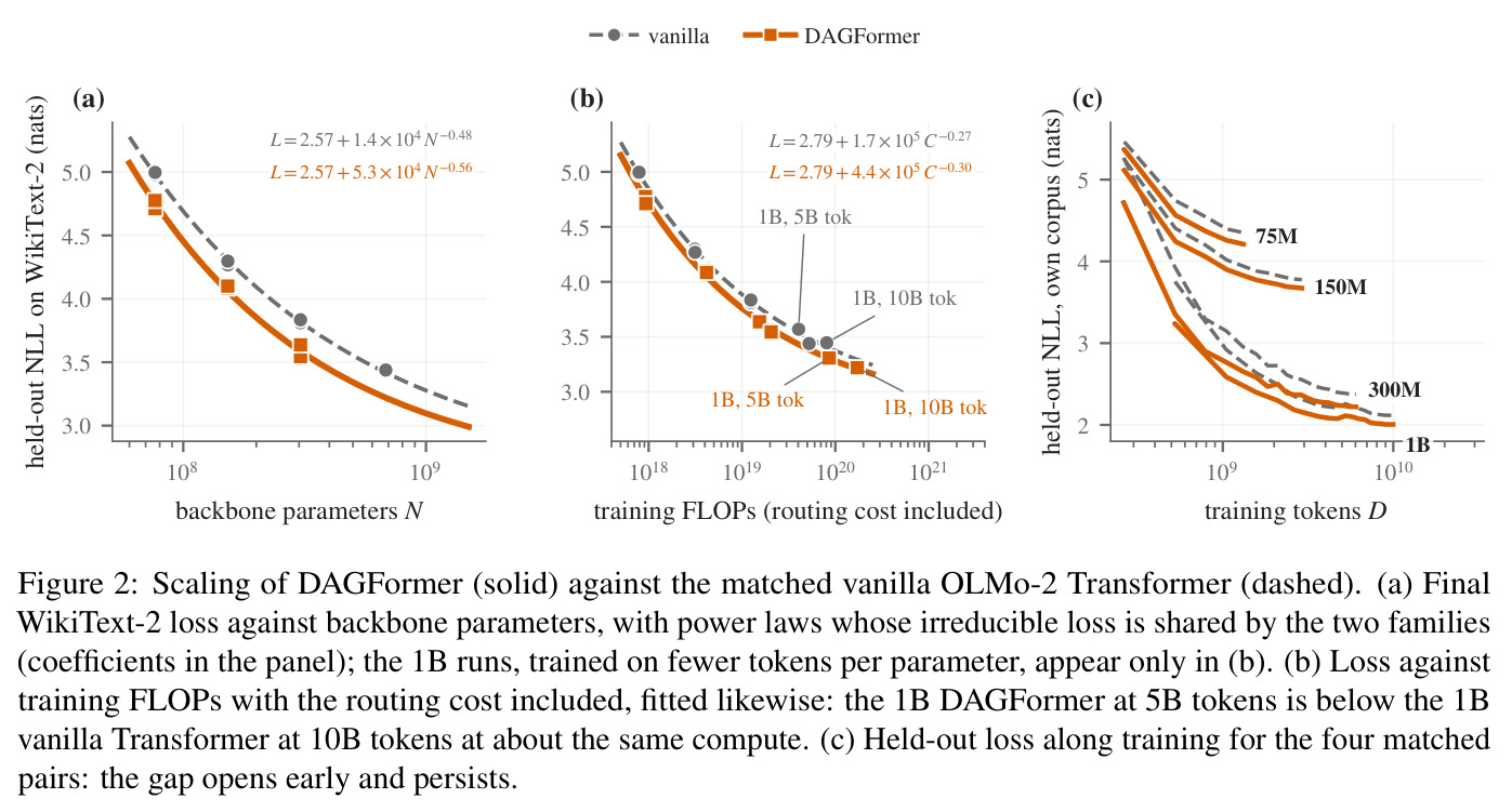
论文用共享 $E$ 的配对拟合证明 DAGFormer 改变了缩放指数（参数 0.56 对 0.48、算力 0.30 对 0.27），这是「架构改进而非多花算力」的关键证据，也是判断其实用价值的依据。

结构化剪枝与泰勒重要性

移除整个注意力头或 MLP 通道而非单个权重。以一阶泰勒展开估计每个单元的重要性（Michel/Molchanov），按渐进立方调度逐步移除并穿插恢复微调；CoFi 即用此套路。

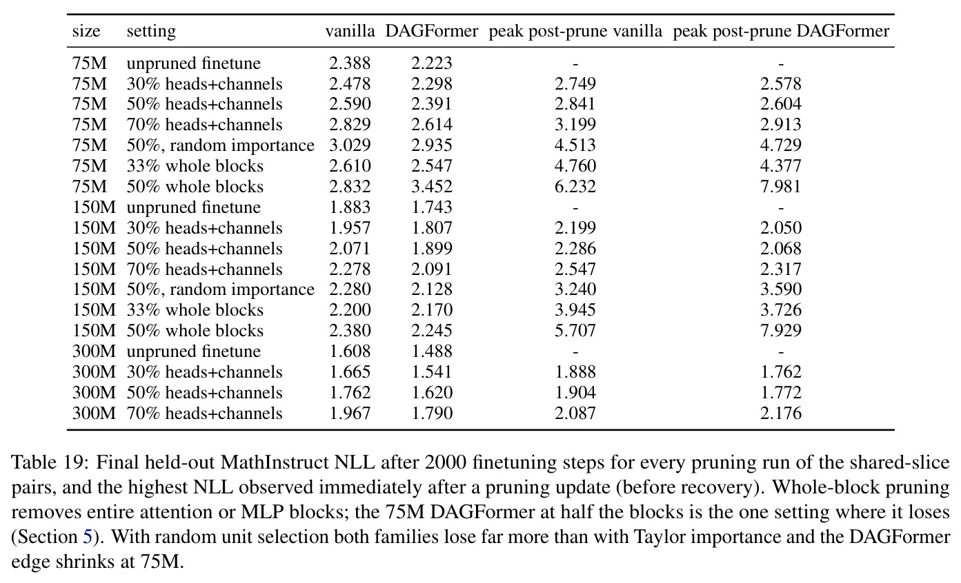
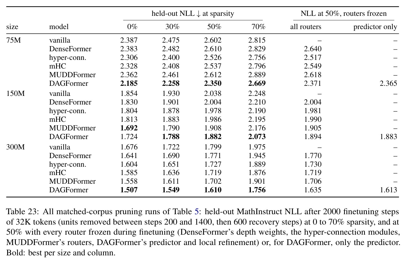
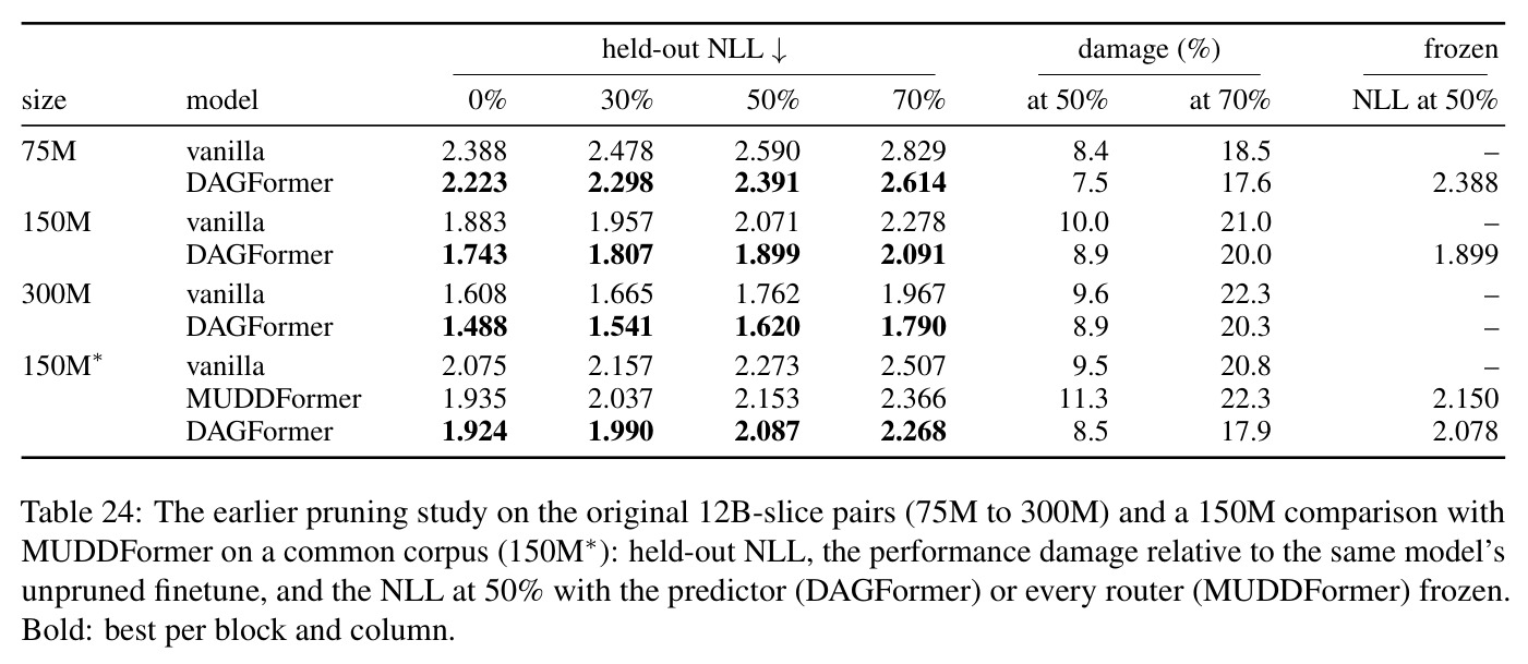
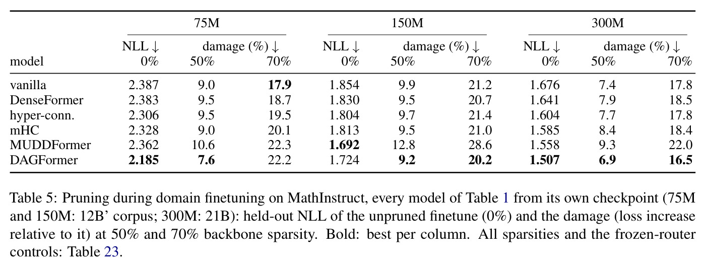
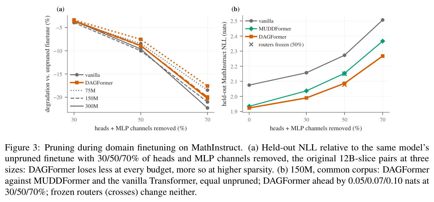
第 5 节用它检验结构收益假设：读取多个早期层的头拥有冗余信息通路，剪掉单元后应退化更慢——这是全局拓扑带来结构鲁棒性的独立证据。

因果（自回归）编码器

只允许关注前缀的编码器：位置 $t$ 的输出只依赖 $x_{\le t}$，不泄漏未来信息，可在自回归解码前独立运行。

拓扑预测器是一个 2 层 4 头、宽 256 的因果编码器；因果性保证每个 token 的连接图不依赖未来 token，模型才能像普通解码器一样从左到右生成。

研究动机

标准 Transformer 通过残差连接组合各层：每个注意力头和 MLP 读写同一条运行和（残差流）。由于带宽被所有层共享，某层能读到哪些早期计算结果完全由结构固定——晚期层只能在「每个中间层都加过自己输出的总和」里看到早期结果。后续工作（DenseFormer、hyper-connections、mHC、MUDDFormer）虽然放开了固定连接、让每层直接读早期层输出甚至按输入逐 token 调整权重，但都做了同一个设计选择：路由是局部的。每层有自己的路由器，读取进入该层的隐状态，决定该层读什么、写到哪；整个模型的跨层拓扑因此是一层一层贪心拼装出来的，没有任何模块对它持有全局视野。其后果有二：跨层协调无法从输入显式规划；拓扑也无法作为一个独立对象被检查、平均或干预。

本文的目标是本文要构建一个跨层连接由「联合训练的拓扑预测器」统一规划的 Transformer 语言模型：预测器只读输入 token，在主干运行之前一次性给出整棵加权有向无环图（DAG），决定每个注意力头和每层残差从哪些早期输出读取、权重多大；每层再用零初始化的局部网络按自身输入修正计划。验证目标很明确：在与 OLMo-2 主干严格配对（同数据序、同 token 预算、同种子、路由算力入账）的 75M–1B 缩放实验中降低损失；战胜 DenseFormer、hyper-connections、mHC、MUDDFormer 四个路由基线；把收益延续到 13 个下游任务、两种指令微调配方与 AlpacaEval；并用结构化剪枝检验学到的拓扑是否带来结构上的鲁棒性。

与已有工作不同的是，独特切入角度是「全局规划 + 局部微调」的分工，而不是再造一个更聪明的逐层路由器。已有动态架构让每层隐状态在本层现场决定读写；DAGFormer 则让一个小型因果编码器只凭 token id 预测整棵图——它看不到任何隐状态，却看到全局深度，因此跨层协调第一次成为可显式规划的对象。这同时把拓扑变成可被平均、冻结、跨样本交换和修补的独立检查点，呼应「生成式可解释性」对推理中干预点的要求。此外混合系数是无约束实数（不像注意力 softmax），读操作可以放大或相减不同来源；且 $W$ 零初始化、$b$ 初始化为选中前一层的 one-hot，使初始时刻严格等价 vanilla Transformer，训练从标准模型平滑出发。

核心方法

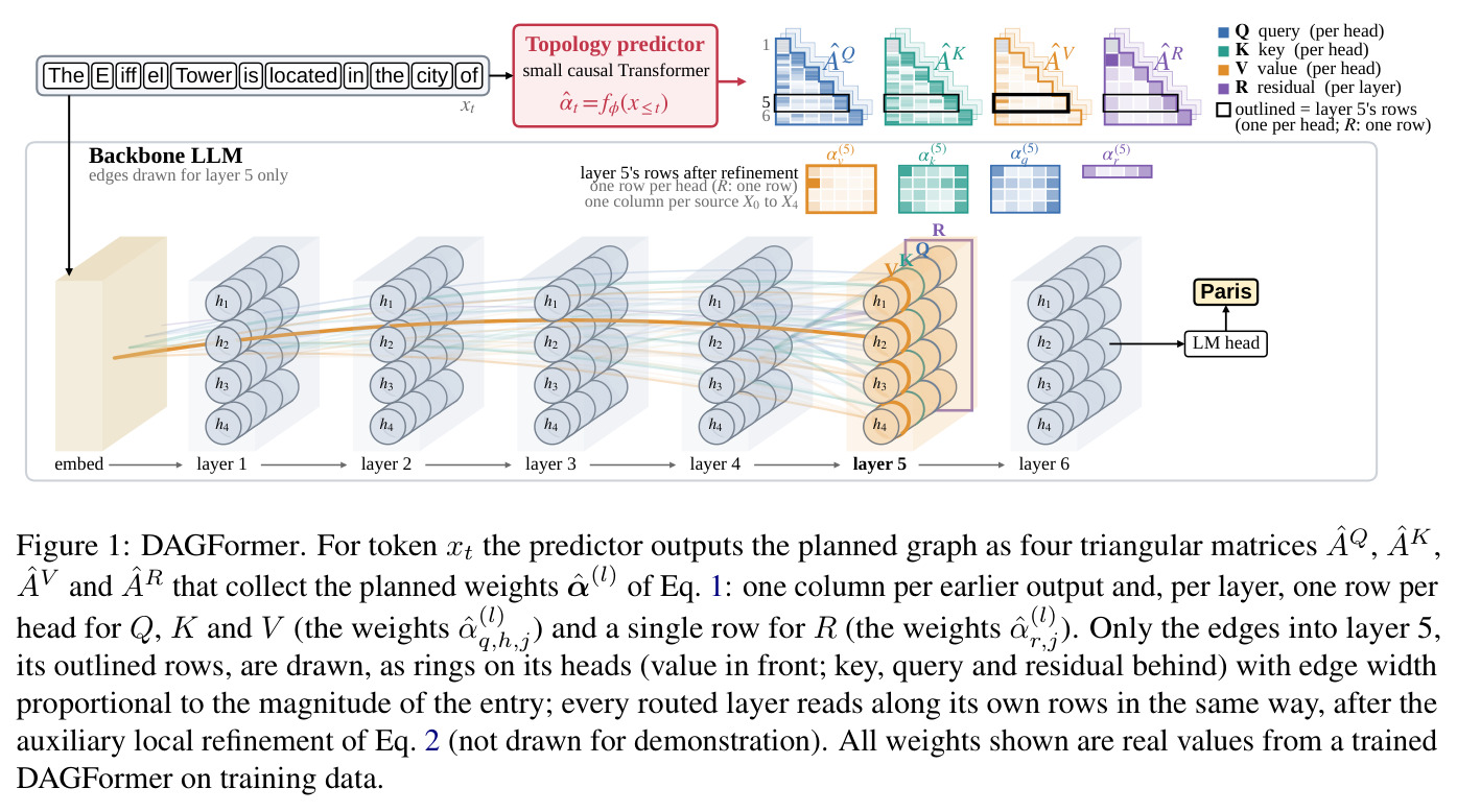
直觉：一个层该读哪些早期结果取决于输入内容——代码、数学、叙事需要不同的信息流。与其让每层各自为战，不如「先看题、再规划」：一个小预测器读完输入前缀，为所有层同时画出一棵加权 DAG，主干沿图计算。技术路线：设 $X_0(t)$ 为 token $t$ 的嵌入，$X_l$ 为第 $l$ 层输出。路由层 $l\ge 2$ 的每个头从 $X_0,\dots,X_{l-1}$ 加权混合出 q、k、v，残差亦然：$q_h=\sum_{j<l}\alpha^{(l)}_{q,h,j}W^q_h X_j$，$R_l=\sum_{j<l}\alpha^{(l)}_{r,j}X_j$；其余模块（Q/K 归一化、MLP、$X_l=R_l+a_l+m_l$）与标准层相同。权重 $\alpha^{(l)}$ 来自预测器的计划 $\hat\alpha^{(l)}=W^{(l)}u+b^{(l)}$（$u=\mathrm{GELU}(W_u\mathrm{LN}(z))\in\mathbb{R}^{512}$），再经零初始化的局部修正 $\alpha^{(l)}=\hat\alpha^{(l)}+W_2^{(l)}\mathrm{GELU}(W_1^{(l)}\mathrm{LN}(X_{l-1}))$。预测器与主干以同一 LM 损失从零联合预训练。

核心创新是用「共享的全局拓扑预测器」取代「逐层路由器」，并配一个只在头粒度做修正的 refinement。本质区别有三。其一，决策视野：hyper-connections、mHC、MUDDFormer 的每层路由器只见进入本层的隐状态，拓扑是贪心拼装；DAGFormer 的预测器读同一份 token id（自配 256 维嵌入、2 层 4 头因果编码器、512 维 trunk），一次性输出全部层的邻接矩阵组 $[\hat A^Q,\hat A^K,\hat A^V,\hat A^R]$，跨层协调可被显式规划。其二，信息不对称的补偿：预测器看不到主干算出的内容，零初始化 refinement 让每层用 $X_{l-1}$ 修正自己每头每读的权重——只修不造，修正量作用于计划而非重新产生计划。其三，稳定性技巧：$W$ 初始化为零、$b$ 每行为选中 $X_{l-1}$ 的 one-hot，初始时刻 DAGFormer 严格等价 vanilla OLMo-2；系数为无约束实数可放大相减；300M/1B 还对混合后的 $v_h$ 施加 RMSNorm（V 归一化）。

方法步骤详情

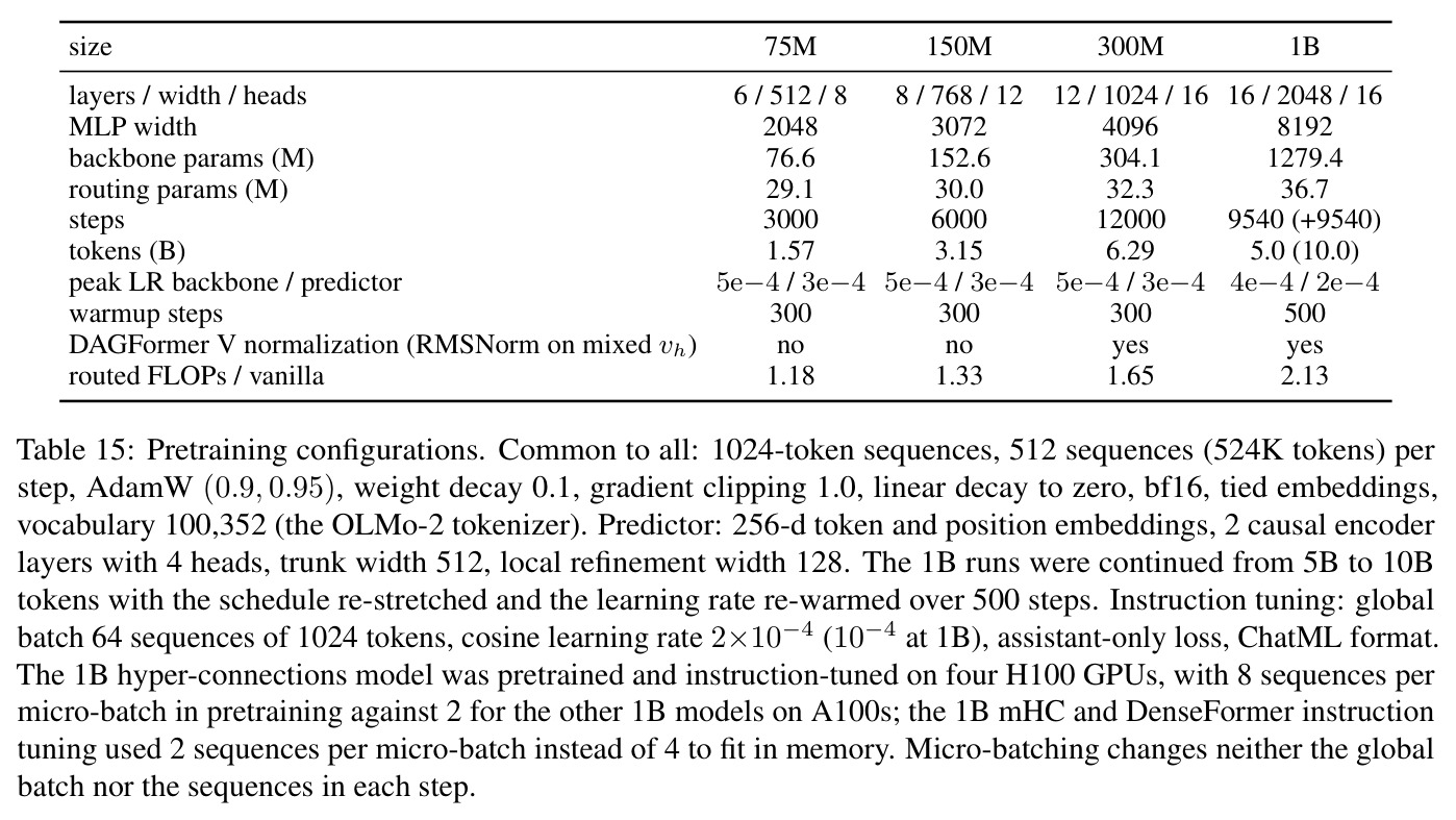
第一步，输入编码：token 序列进入拓扑预测器——256 维 token/位置嵌入，2 层 4 头因果编码器，输出 $z$；因果性保证每个 token 的图不依赖未来 token，可从左到右生成。第二步，图预测：$u=\mathrm{GELU}(W_u\mathrm{LN}(z))\in\mathbb{R}^{512}$ 的共享 trunk 后，每个路由层接线性头 $\hat\alpha^{(l)}=W^{(l)}u+b^{(l)}$，$W^{(l)}\in\mathbb{R}^{(3H+1)l\times512}$，重排为该层 $3H{+}1$ 行（每头 q/k/v 各一行、残差一行）$\times\, l$ 列（每个早期源一列）的计划矩阵。第三步，局部修正：refinement（$W_1\in\mathbb{R}^{128\times D}$、$W_2\in\mathbb{R}^{(3H+1)l\times128}$，零初始化，不足前向 MAC 的 0.5%）从 $X_{l-1}$ 算出加性修正，得最终 $\alpha^{(l)}$。第四步，沿图计算：路由层把 $l$ 个源堆叠过一次融合 q/k/v 投影再加权和，第 1 层不路由，其余模块照旧。第五步，联合训练：预测器与主干从零预训练，预测器学习率为主干的 0.6 倍。配置：75M=6层/D512/H8、150M=8/768/12、300M=12/1024/16、1B=16/2048/16，路由参数 29M–37M（含 25.7M 共享预测器词嵌入），数据 Dolma v1.7，每步 524K token，75M–300M 约 21 token/参数。

技术新颖性

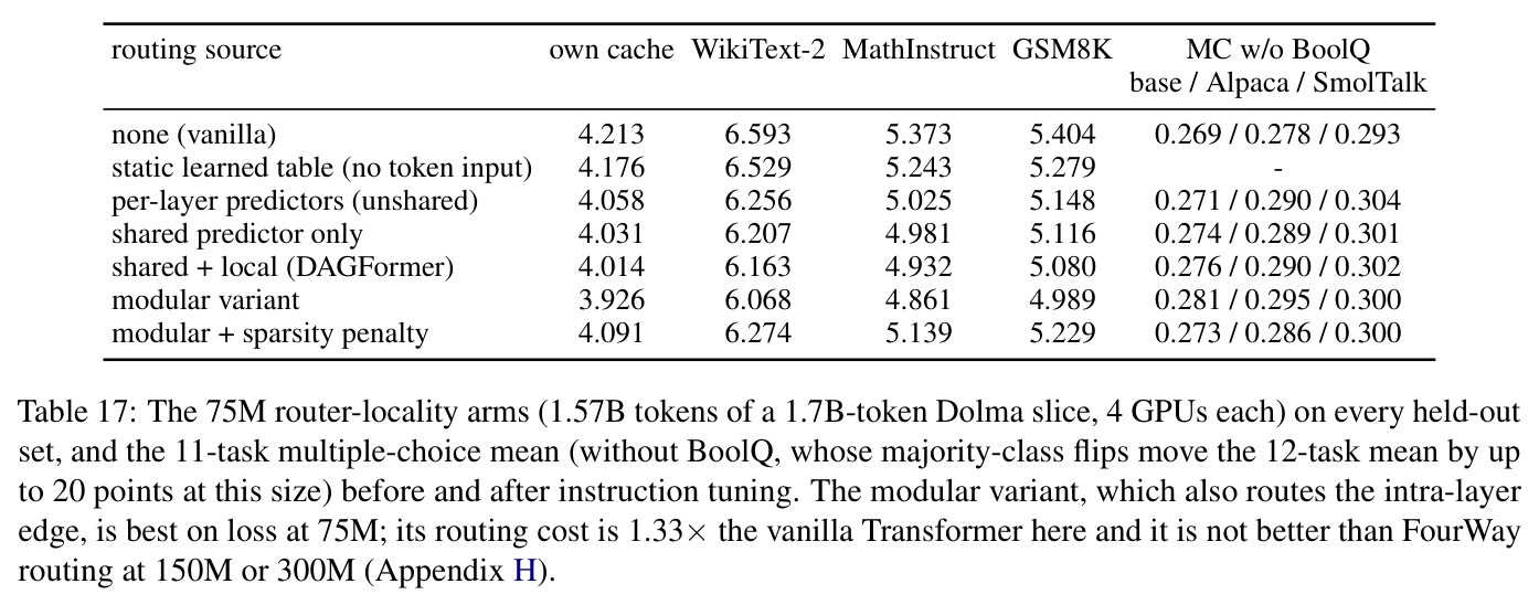
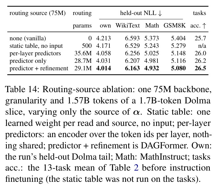
技术新颖性有四点。(1) 全局性：首个用单一模块在主干运行前预测整棵跨层连接图的 Transformer 变体。最近类比 BlockDrop 也用一个策略网络为图像一次选块，但它选择跳过哪些块（改变计算量），DAGFormer 保持计算量固定、只选每层读哪些源——与 MoE/早退等条件计算正交。(2) 规划/执行解耦：预测器输出是可审计对象，可做平均、冻结、跨窗口交换等因果干预（附录 D/E 正是用它们定位收益来源），逐层路由器在结构上做不到。(3) 参数化自带归纳偏置：消融显示「用 token 学出一张（近乎静态的）图」贡献约 90% 收益，而直接训练的无输入静态表只能恢复 17–23%，说明收益来自参数化方式而非逐 token 重规划。(4) 与 MUDDFormer 共享「每头 q/k/v 分解」，但把「每层隐状态生成权重」改为「一个编码器为所有层生成 + 每层 refinement 修正」；实验显示共享预测器优于每层独立预测器（恢复不足 80%，还多花 7M 参数）。

**Figure 1**: DAGFormer. For token $x_t$ the predictor outputs the planned graph as four triangular matrices $\hat A^Q$, $\hat A^K$, $\hat A^V$ and $\hat A^R$ that collect the planned weights $\hat\alpha^{(l)}$ of Eq. 1: one column per earlier output and, per layer, one row per head for Q, K and V and a single row for R. All weights shown are real values from a trained DAGFormer on training data.

实验结果

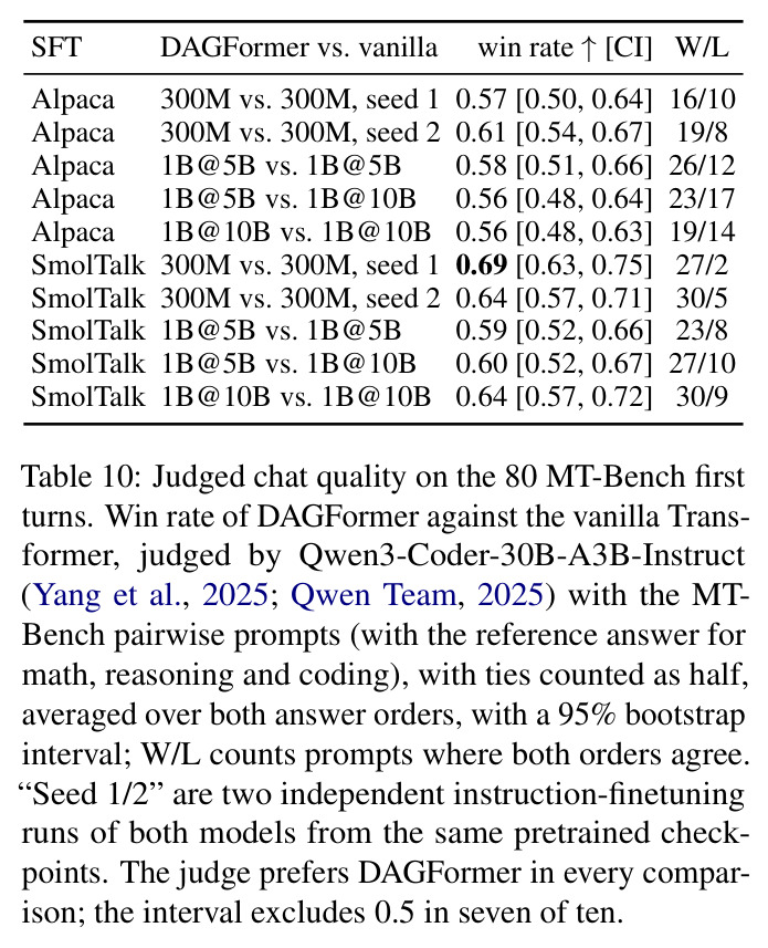
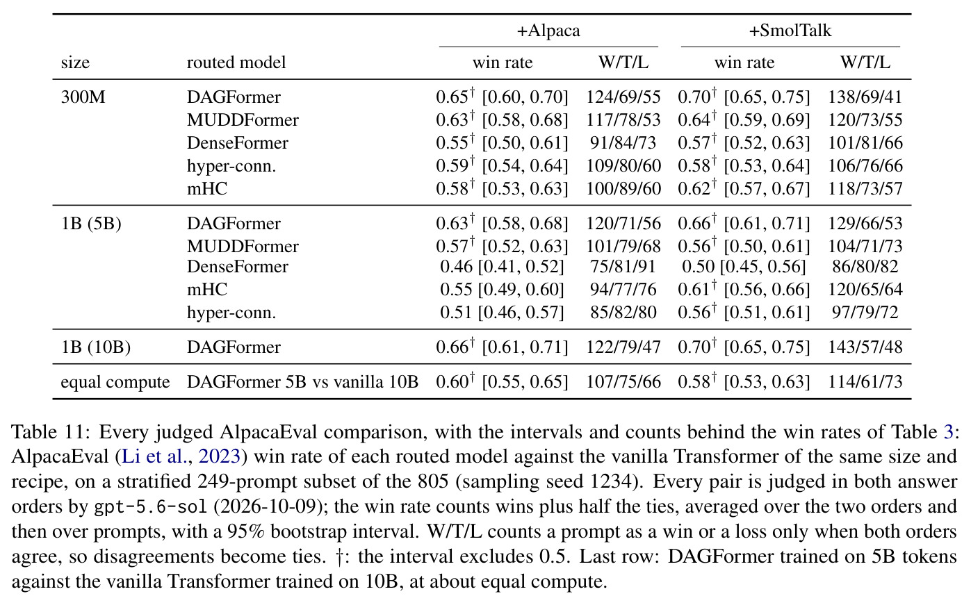
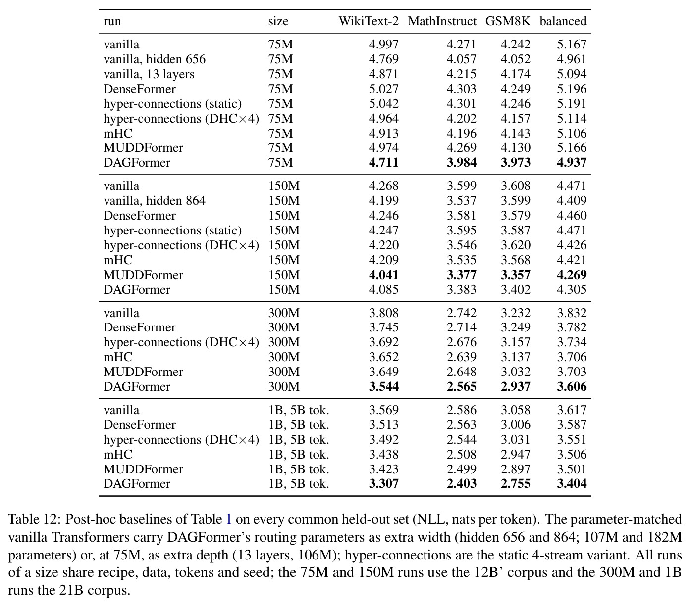
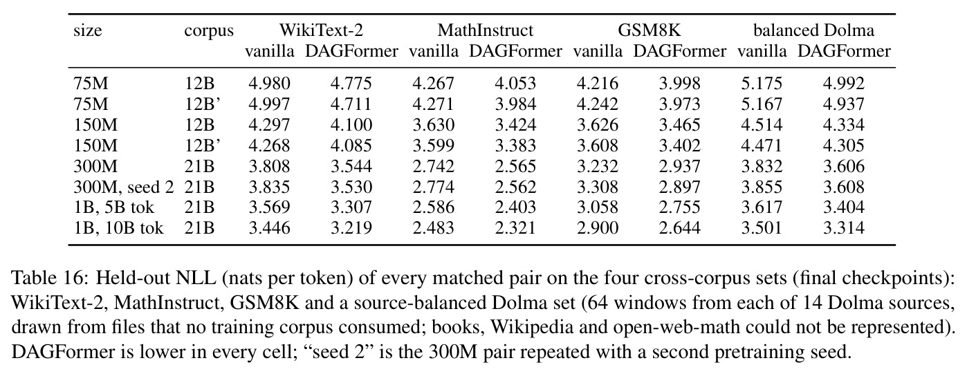
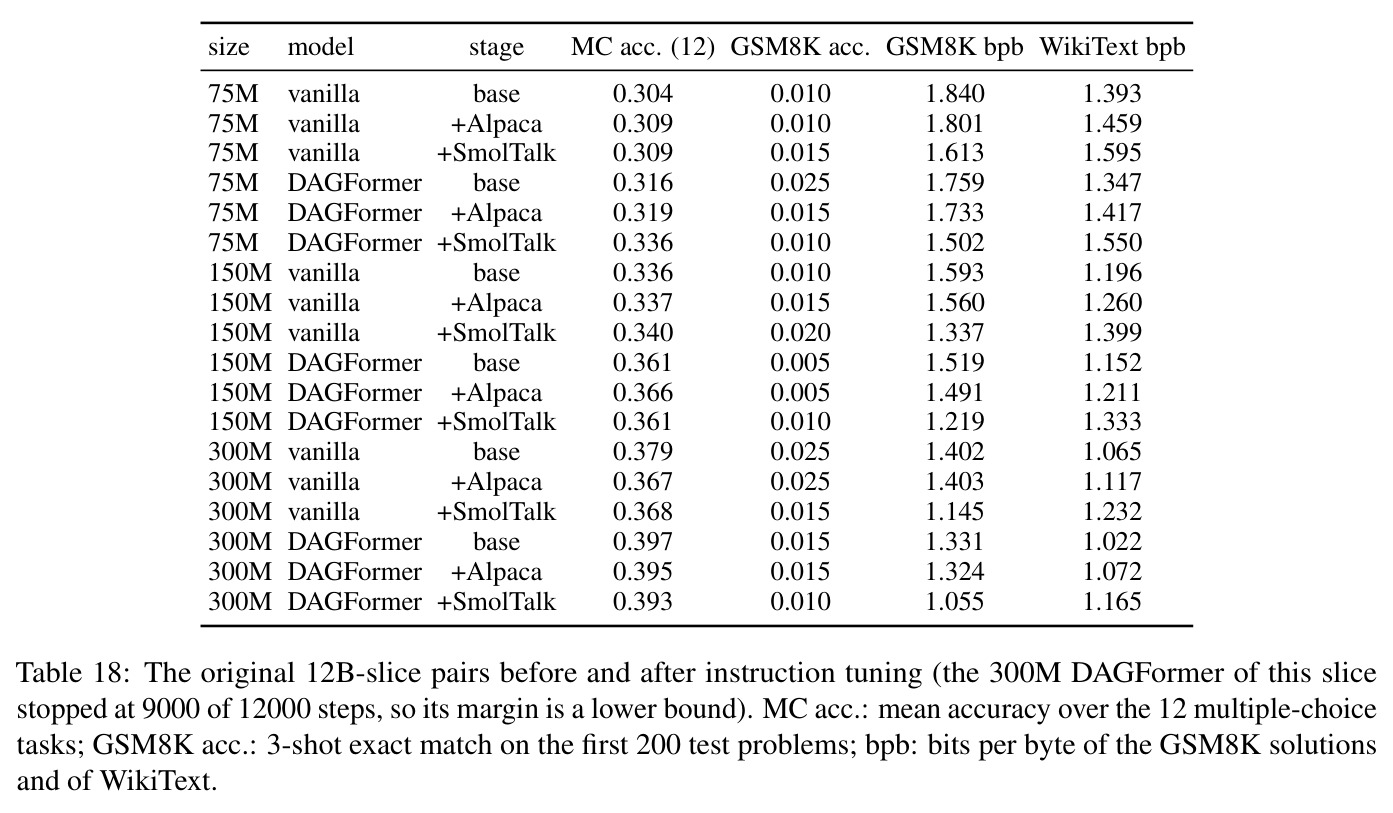
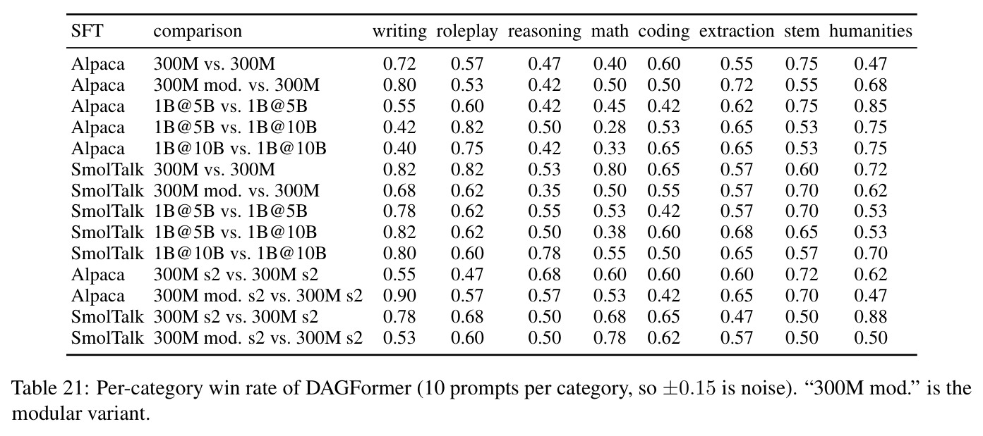
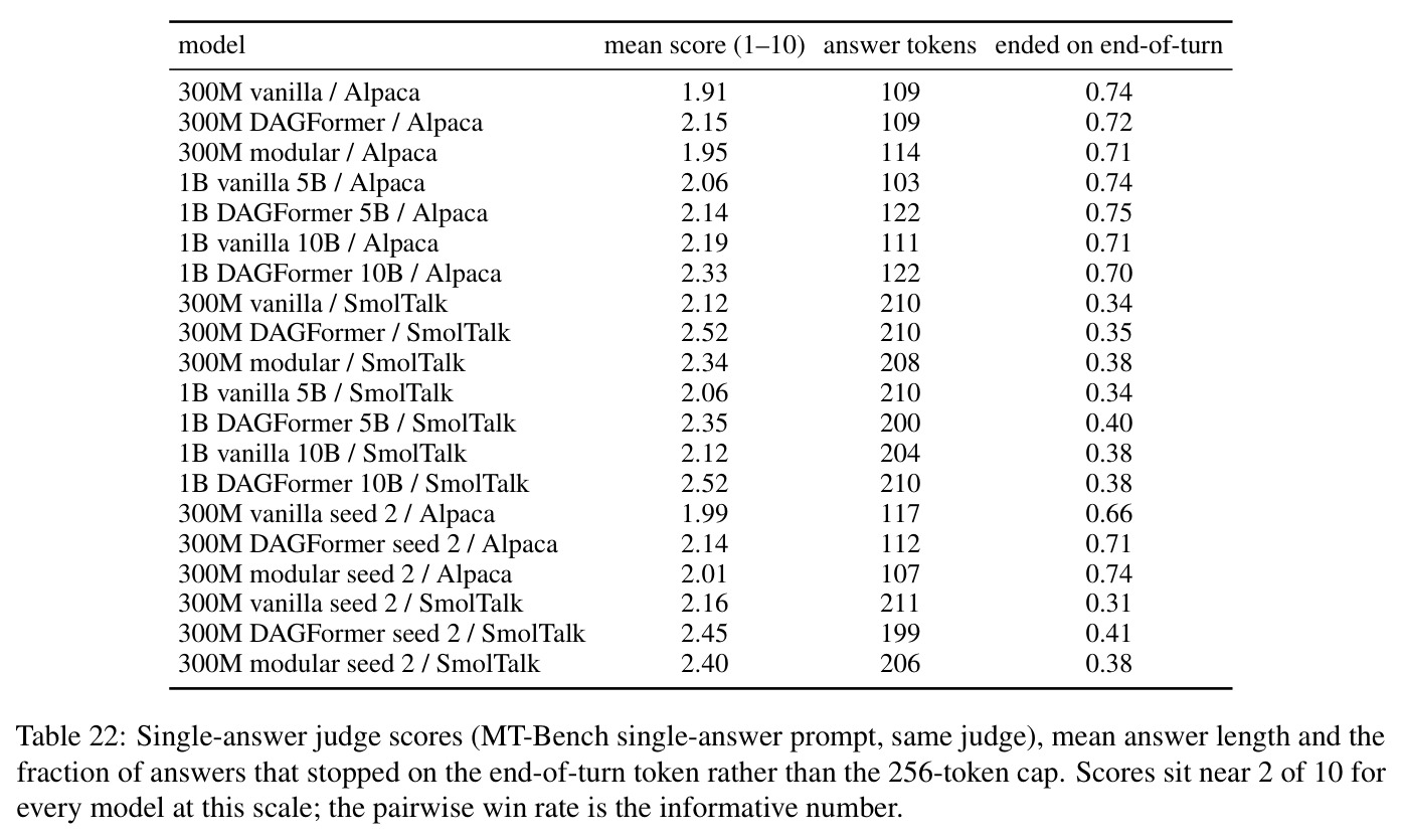
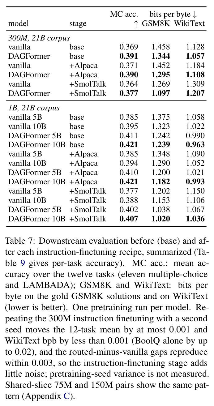
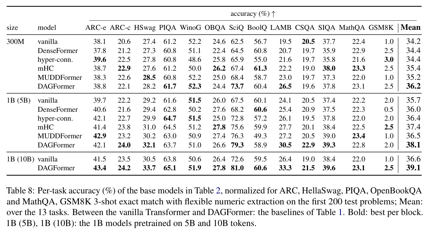
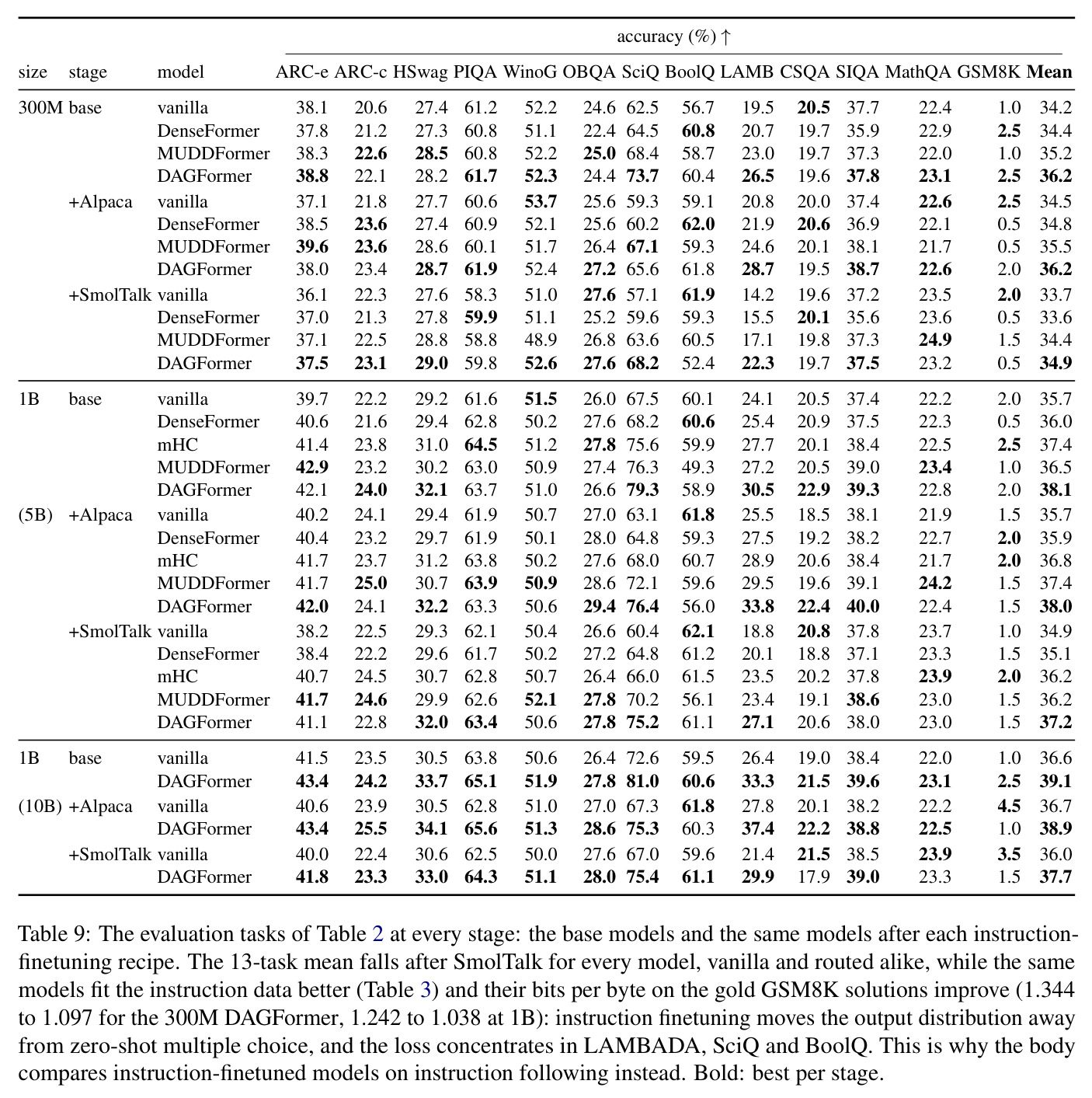
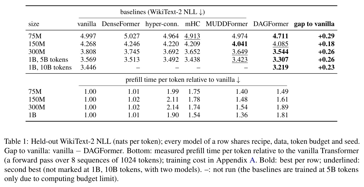
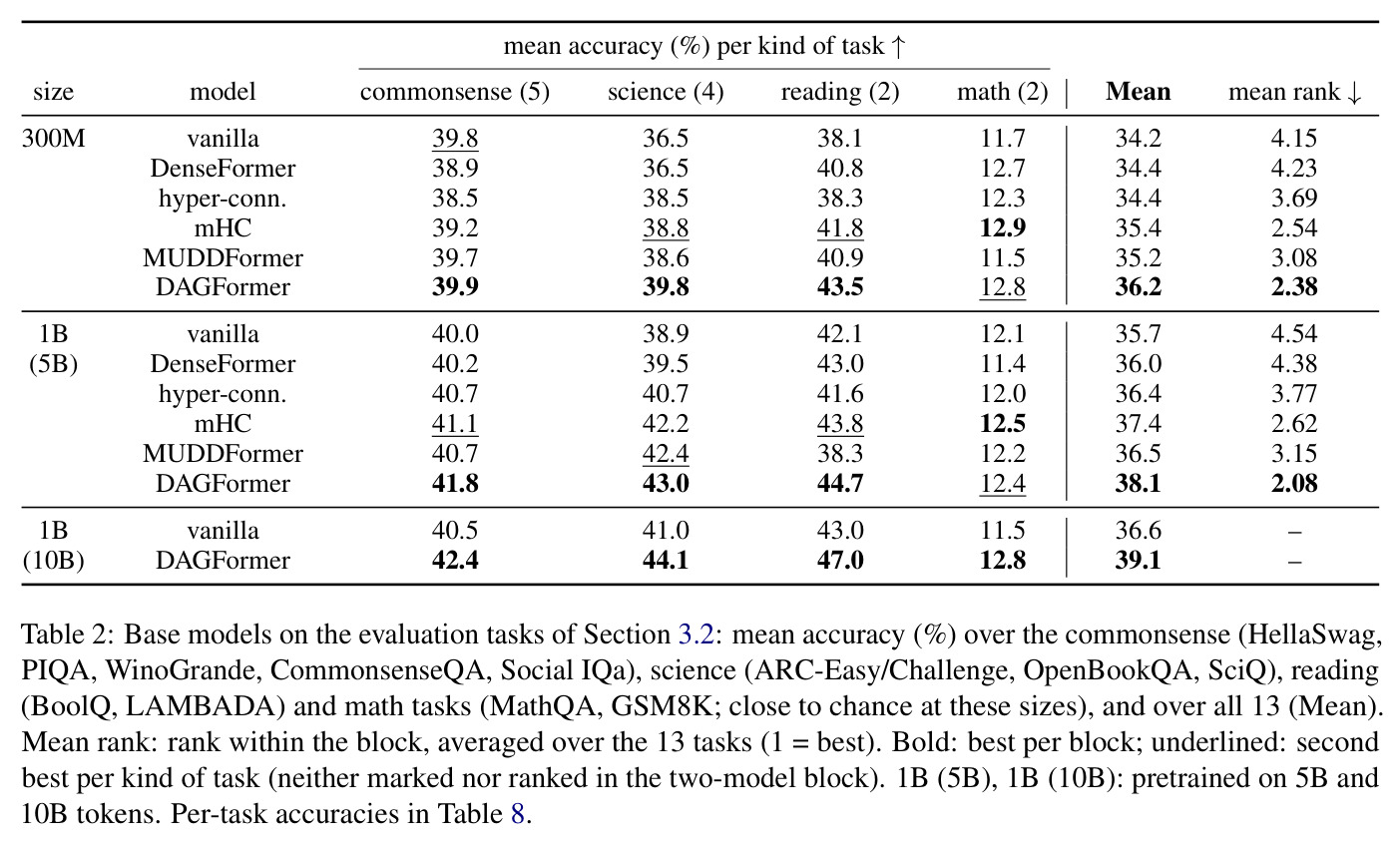
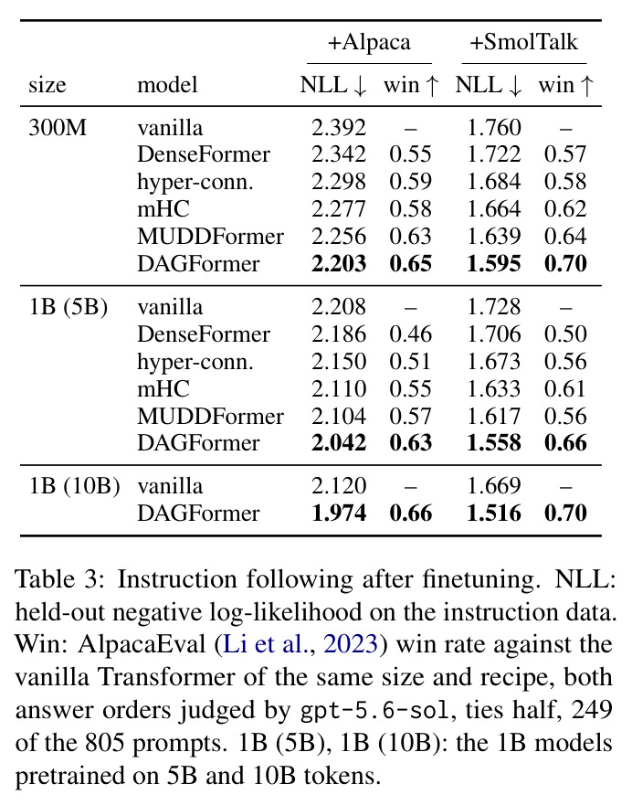
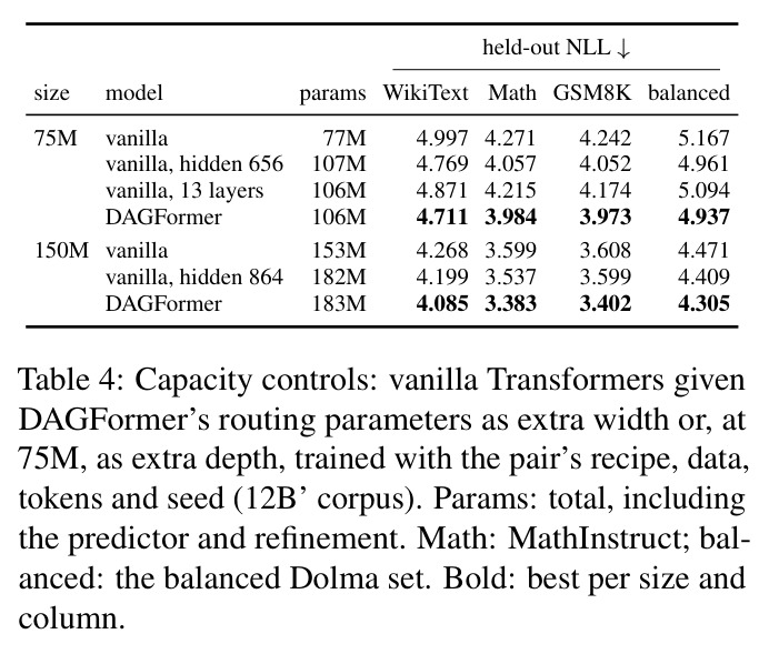
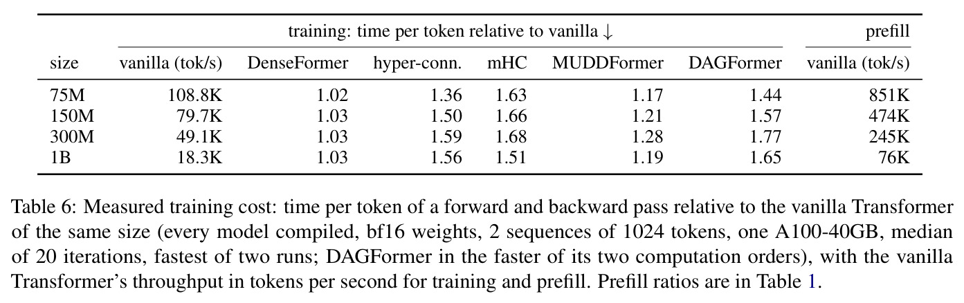
逐项看实验。主结果（Table 1）：WikiText-2 NLL 上 DAGFormer 把配对成绩从 4.997 降到 4.711（75M）、4.268→4.085（150M）、3.808→3.544（300M）、3.569→3.307（1B@5B）、3.446→3.219（1B@10B），比 vanilla 低 0.18–0.29 nats（困惑度低 17%–25%），并在 75M、300M、1B 同时是所有路由基线中最低，仅 150M 被 MUDDFormer 以 0.04 nats 反超。等算力下 1B DAGFormer@5B token 全面超过 1B vanilla@10B token（3.307 对 3.446；MathInstruct 2.403 对 2.483；GSM8K 2.755 对 2.900）。缩放拟合（Figure 2）：共享不可约损失下指数更大——参数 0.56 对 0.48、算力 0.30 对 0.27；vanilla 需 1.2–1.4 倍（小模型）至 1.7–2.0 倍（300M/1B）算力才能追平。下游 13 任务（Table 2）：均值 36.2 对 34.2（300M）、38.1 对 35.7（1B@5B）、39.1 对 36.6（1B@10B），领先最强基线 0.7–0.8 点，平均排名 2.38/2.08。指令微调（Table 3）：held-out NLL 比 vanilla 低 0.15–0.19 nats、比最强基线低 0.04–0.06；AlpacaEval 胜率 0.63–0.70（基线 0.46–0.64）；MT-Bench 胜率 0.56–0.69。剪枝（Table 5）：六设置中五者退化最小，50% 稀疏度损伤 6.9%–9.2%（MUDDFormer 9.3%–12.8%），冻结路由几乎不变。代价：FLOPs 1.18–2.13 倍，实测训练时间 1.44–1.77 倍。

**Table 1**: Held-out WikiText-2 NLL (nats per token); every model of a row shares recipe, data, token budget and seed. Bottom: measured prefill time per token relative to the vanilla Transformer. Gap to vanilla: vanilla − DAGFormer.

**Table 2**: Base models on the evaluation tasks: mean accuracy (%) over commonsense (5), science (4), reading (2) and math (2) tasks, and over all 13; mean rank within each block.

**Table 3**: Instruction following after finetuning. NLL: held-out negative log-likelihood on the instruction data. Win: AlpacaEval win rate against the vanilla Transformer of the same size and recipe, both answer orders judged by gpt-5.6-sol, 249 of the 805 prompts.

**Table 4**: Capacity controls: vanilla Transformers given DAGFormer's routing parameters as extra width or, at 75M, as extra depth, trained with the pair's recipe, data, tokens and seed.

**Table 5**: Pruning during domain finetuning on MathInstruct: held-out NLL of the unpruned finetune (0%) and the damage (loss increase relative to it) at 50% and 70% backbone sparsity.

**Table 6**: Measured training cost: time per token of a forward and backward pass relative to the vanilla Transformer of the same size (compiled, bf16, 2 sequences of 1024 tokens, one A100-40GB), with the vanilla Transformer's throughput in tokens per second.

**Table 14**: Routing-source ablation: one 75M backbone, varying only the source of $\alpha$. Static table: one learned weight per read and source, no input; per-layer predictors: an encoder over the token ids per layer, nothing shared; predictor + refinement is DAGFormer.

**Table 20**: Held-out NLL when one routing channel is replaced by its mean over 128 held-out windows of the model's own corpus.

**Figure 2**: Scaling of DAGFormer (solid) against the matched vanilla OLMo-2 Transformer (dashed): (a) final WikiText-2 loss against backbone parameters with power laws sharing the irreducible loss; (b) loss against training FLOPs with the routing cost included; (c) held-out loss along training for the four matched pairs.

**Figure 3**: Pruning during domain finetuning on MathInstruct: (a) held-out NLL relative to the same model's unpruned finetune with 30/50/70% of heads and MLP channels removed; (b) 150M, common corpus: DAGFormer against MUDDFormer and the vanilla Transformer, with frozen-router controls.

**Figure 4**: The modular variant against DAGFormer (FourWay routing) and the vanilla OLMo-2 Transformer: (a) final WikiText-2 loss against backbone parameters, (b) against training FLOPs with the routing cost included.

查看结构化数据

任务	指标	本文	基线	提升
语言建模 WikiText-2（75M 配对）	NLL（nats/token）↓	4.711	vanilla 4.997；最佳基线 mHC 4.913	较 vanilla −0.29 nats（困惑度 −25%），较最佳基线 −0.20
语言建模 WikiText-2（300M 配对）	NLL ↓	3.544	vanilla 3.808；最佳基线 MUDDFormer 3.649	较 vanilla −0.26，较最佳基线 −0.11
语言建模 WikiText-2（1B，5B token）	NLL ↓	3.307	vanilla 3.569；最佳基线 MUDDFormer 3.423	较 vanilla −0.26，较最佳基线 −0.12
等算力对比：1B DAGFormer@5B token 对 1B vanilla@10B token	三个 held-out 集平均 NLL	WikiText-2 3.307 / MathInstruct 2.403 / GSM8K 2.755	vanilla@10B：3.446 / 2.483 / 2.900	约相同训练算力下全面更低（−0.14/−0.08/−0.15 nats）
13 个下游任务均值（300M 与 1B@5B）	平均准确率（%）↑，及 13 任务平均排名 ↓	36.2（排名 2.38）；1B@5B 38.1（排名 2.08）	vanilla 34.2 / 35.7；最佳基线 mHC 35.4 / 37.4	较 vanilla +2.0/+2.4 点，较最佳基线 +0.8/+0.7 点
指令微调后 AlpacaEval（805 题分层抽 249 题，gpt-5.6-sol 双序评判）	对同规模 vanilla 的胜率 ↑	0.63–0.70（各规模两种配方全部显著）	路由基线 0.46–0.64；1B DenseFormer 0.46 不显著	高于所有路由基线约 0.04–0.17
结构化剪枝（MathInstruct 域微调，剪头+MLP 通道）	50% 稀疏度下相对自身未剪模型的损失损伤（%）↓	7.6 / 9.2 / 6.9（75M/150M/300M）	vanilla 9.0/9.9/7.4；MUDDFormer 10.6/12.8/9.3	六设置中五者退化最小；冻结路由器结果几乎不变
算力开销（对比侧）	相对 vanilla 的 FLOPs 倍数 / 实测训练时间倍数	1.18–2.13× FLOPs；1.44–1.77× 实测训练时间	MUDDFormer 1.17–1.28× 时间；hyper-connections 1.36–1.59×；mHC 1.51–1.68×	更贵，但 vanilla 需 1.7–2.0× 算力才能在 300M/1B 追平损失

局限与改进

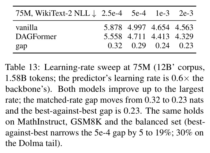
作者承认的局限：最大仅 1B、训练 5–10B token，低于计算最优预算；除 300M 外全是单种子，而换种子可移动高达 0.08 nats（WikiText-2 上至多 0.03），更小的差异可能是噪声；剪枝也是单次运行；150M 上 MUDDFormer 以 0.04 nats 胜出，单种子无法定论；1B 基线只有 5B token 版本、参数匹配对照只有 75M/150M、学习率扫描只在 75M 做过；该规模模型在难基准接近随机，聊天评测依赖单一 LLM 裁判；可解释性上只以聚合方式读图，逐输入的图是否有可命名含义尚属开放。我的补充：成本随深度近似二次增长（路由 FLOPs 含 $\sum_{l\ge2}(l-1)\cdot3D^2$，1B 已 2.13×，更深会更贵）；峰值内存明显更高（1B 推理 9.1 对 4.2 GB）；训练好的模型依赖 refinement 的逐 token 修正，不能以固定拓扑直接部署；实验仅英语语料，未与 MoE 等正交方法组合验证。

独立分析的弱点

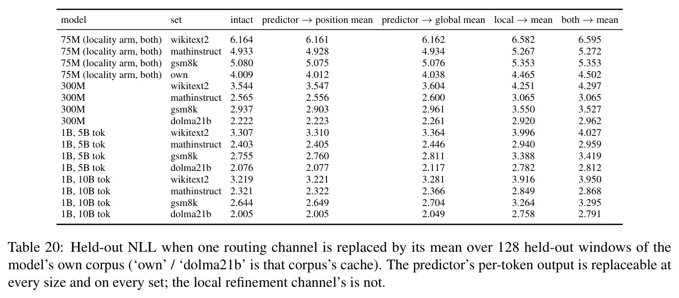
独立分析的弱点：(1) 深度二次成本——路由 FLOPs 含 $\sum_{l\ge2}(l-1)\cdot3D^2$，随层数平方增长；论文自己证明 mix-then-project 顺序理论上只需 1.02–1.04× 却受内存带宽限制，出路是融合 kernel 或稀疏/分块规划，而非算法层回避。(2) 「动态」卖点名不副实——预测器输出可被逐位置均值替换而几乎无损（≤0.005 nats），跨窗口交换仅动 ≤0.007 nats，说明模型学到的是静态图，逐 token 预测机制利用率很低；可退化为「按域/任务选图」的轻量模块。(3) refinement 不可压缩——替换成均值损失 0.27–0.75 nats，抹掉均值 |α| 最小的四分之一条目就损失 0.27–0.4 nats，阻碍部署优化与图稀疏化。(4) 150M 输给 MUDDFormer 且无多种子确认，「全面领先」的稳健性打折扣。(5) 剪枝优势在随机移除下明显缩小，说明依赖泰勒重要性排序，「多通路冗余」假设未被直接检验。(6) 25.7M 的预测器词嵌入对 75M 主干是约三分之一额外参数，嵌入共享值得尝试。

未来方向

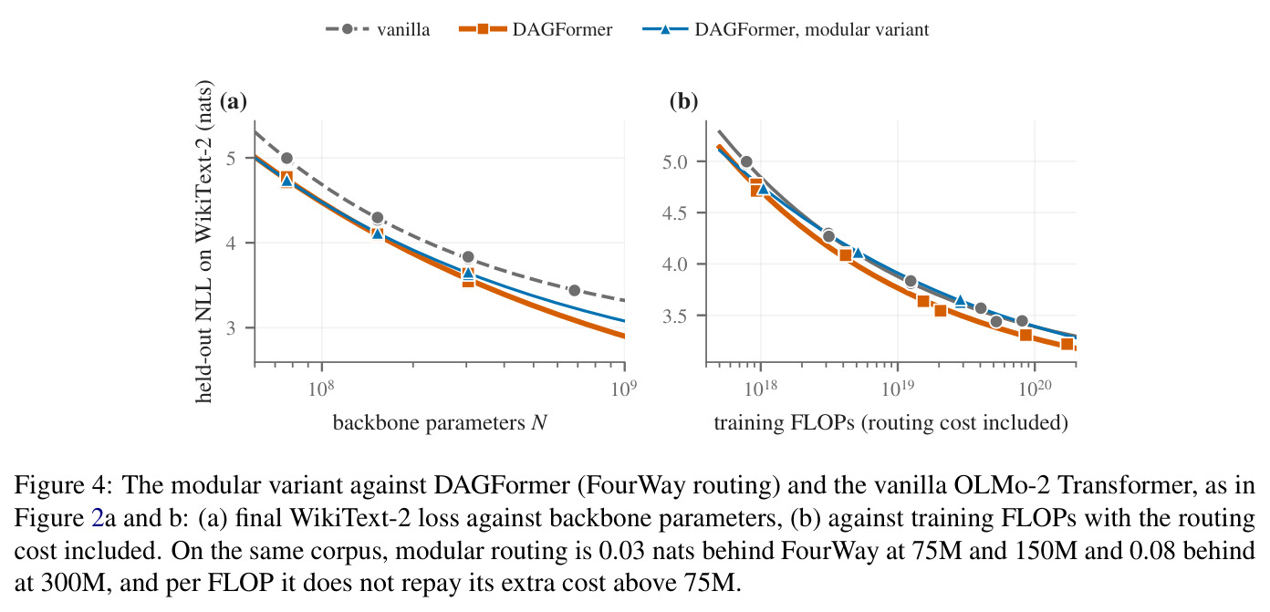
作者提出的方向：把学到的图蒸馏成固定拓扑、用稠密 kernel 高效执行（后验稀疏化代价高，需重训）；训练一个更大的「仅预测器」DAGFormer，使图以可命名方式（任务、领域）随输入变化，让拓扑成为生成式可解释性的推理中检查点；在模块化变体（路由到注意力/MLP 模块级输出）基础上实现专用模块间的路由。基于成果可延伸的：(1) 与 MoE、早退组合——DAGFormer 路由「读什么」而非「算多少」，两类方法正交；(2) 深度扩展——trunk 固定 512 维、加深主干只需加线性头，检验 7B+ 是否保持指数优势；(3) 为混合实现手写 kernel，把推理开销压向 1.05×；(4) 在多语言/多域语料上检验学到的图是否按域分化并可视化；(5) 把图平均/交换用作机制可解释性的标准干预工具（附录 D/E 已示范），与 circuit 分析衔接。

复现评估

复现友好度较高。架构基于 HuggingFace Transformers 的 OLMo-2 实现与分词器（Apache 2.0），全部从随机初始化训练；数据 Dolma v1.7、Alpaca-cleaned、Dolly、smol-smoltalk 均公开；评测用 lm-evaluation-harness 0.4.13；Table 15 给出全部超参（AdamW (0.9,0.95)、wd 0.1、clip 1.0、bf16、1024 token 序列、每步 524K token、学习率 5e-4/3e-4、预测器 0.6 倍学习率）。总算力约 3,700 GPU 小时（2,250 A100-40GB、510 A40、470 A5000、350 A6000、80 H100），单卡 A100 即可复现 75M–300M 配对（75M 吞吐 108.8K tok/s），1B 需 4 卡级资源。坑点：hyper-connections 无官方代码（作者用 lucidrains 实现），mHC 用 DeepSeek 官方参考算子；DAGFormer 无手写 kernel，需 torch.compile 才能达报告速度，且推理默认保留所有层输出（1B 峰值 9.1 GB）；论文未给出明确的代码/权重发布链接，需自行实现。