← 返回 2026-10-12

AMLworld-Compact:重要性加权降采样实现低成本的 LLM 评估与错误诊断 AMLworld-Compact: Importance-Weighted Downsampling for Cost-Effective LLM Evaluation and Error Diagnosis

Natapong Nitarach, Phume Ngampornsukswadi, Pittawat Taveekitworachai, Surapon Nonesung, Warit Sirichotedumrong, Kunat Pipatanakul 📅 2026-10-09 👍 13 2026-10-20 18:30
Horvitz-Thompson估计 LLM评估 反洗钱 图文本序列化 重要性加权采样 错误诊断

保留全部非法交易并加权采样合法交易,将百万级测试评估压缩 271–611 倍且可无偏估计全量指标

前置知识

Horvitz–Thompson (HT) 估计

调查抽样中的经典设计基(design-based)估计量:若总体单元 $i$ 以已知入样概率 $\pi_i$ 被抽中,则总量 $T$ 的估计为 $\hat{T}=\sum_{i\in S} z_i/\pi_i$,权重 $w=1/\pi$。在预测向量固定时其期望等于真值,即无偏;分层抽样中层内权重为 $N_h/n_h$。它是本文把小子集指标还原为全测试指标的数学基础。

论文的核心主张——'271–611 倍压缩后仍能无偏估计全测试混淆计数'、发布入样权重、构造保守置信区间——全部建立在 HT 估计之上;不理解它就无法理解为何 3,753 个目标能代表 101 万条边。

混淆矩阵与精确率/召回率/F1

二分类评估的基本工具:TP/FP/FN/TN 四个计数派生出精确率 $P=TP/(TP+FP)$、召回率 $R=TP/(TP+FN)$ 与 $F_1=2PR/(P+R)$。本文中召回只涉及非法边(全部保留、权重为 1),因此可精确计算;而 $P$ 与 $F_1$ 是两个加权计数之比,属比值估计量,有限样本下存在偏差与方差。

论文反复强调'召回精确、P/F1 是比值估计'这一区分,并以此解释为何置信区间宽达数十个百分点;读懂误差分析必须熟悉这些指标的计数构成。

分层抽样与难负样本(hard negatives)

把总体按辅助信息分成同质层,再在每层内独立抽样以降低方差;Neyman 分配按层内方差最优分配样本量。难负样本指监督模型打分接近阈值、极易被误判为非法的合法交易,本文用难度分数 $d(e)=1-2|\bar{p}(e)-0.5|$ 度量($\bar{p}=0.5$ 时最难),并把合法预算集中到这一层。

HT-Coreset 的合法预算分配(最多 30% 给难负层 + 三个难度三分位层)以及 B5 Neyman 分配对照、B4 去难负层消融,全部围绕这些概念展开。

AMLworld 数据集与洗钱类型学(typology)

Altman 等人 2023 年发布的合成反洗钱交易图基准,交易表示为带标签的边,非法边可标注 8 种洗钱模式:fan-out、fan-in、cycle、scatter-gather、gather-scatter、stack、bipartite、random。HI-Small 与 LI-Small 是其两个最小切分,测试集非法率分别约 0.12% 和 0.05%。

评估集的构造对象、类型学宏 F1(TF1)指标、以及'保留全部非法边即保留全部 8 类模式'的论证都依赖该数据集的结构;类型学分布(如 gather-scatter 占 32.7%)也出现在诊断分析中。

GFP 特征与梯度提升树集成

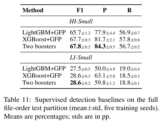
Graph Feature Preprocessor(Blanuša 等 2024)从子图实时提取特征(本文 73 维 GFP + 6 个原始属性),供 LightGBM/XGBoost 等梯度提升树做边分类。本文用 3 个 scorer × 5 个训练 seed 的平均概率 $\bar{p}(e)$ 定义难度分层,并以 LightGBM+XGBoost 双 booster 集成(阈值 0.80/0.48)作为 ML 参照(HI-Small 全测试 F1 68.1%)。

分层构造、ML–LLM 错误重叠分析、held-out 验证设计都以这些监督模型为核心;'指标精确一致'的结论只对参与分层的构造集成成立。

k-hop 类型化图序列化(typed-graph serialization)

把图邻域转成 LLM 可读文本:从目标交易的源账户出发做 BFS 到深度 $k=2$,每跳最多取 50 个未访问邻居;账户/银行是带类型节点,转账/银行成员是带类型关系,交易属性(金额、币种、支付方式、时间戳)写入文本;few-shot 版本前置 12 个演示(约 30K token)。

这是被评估 LLM 的实际输入。论文发现 324/297 个案例的目标交易在上下文中缺席、目标未标记、单次全量评估约 68M/42M token 等关键问题都源于这种序列化方式。

研究动机

反洗钱(AML)检测要判断一笔交易是否属于非法活动,证据往往横跨多个账户与转账(如 gather-scatter 模式先汇集资金再分散)。用 LLM 评估时,每个交易目标都需要一条独立的图 prompt:AMLworld 两个最小切分的测试集 HI-Small 与 LI-Small 分别含 1,015,669 与 1,384,810 条边,非法率仅 0.12% 与 0.05%,单次完整评估需要超过一百万条图 prompt,仅图文本就约 68M/42M token,比较多个模型和 prompt 变体会成倍放大成本。类比例的均衡采样虽能提高非法样本占比,却改变了无加权精确率和 F1:在 1:2 子集上'全部预测非法'的精确率是 33.3%、F1 是 50.0%,而全量 HI-Small 测试上仅 0.123% 与 0.246%。先前的探索性工作(Pirmorad, 2025)在小规模均衡 AMLworld 子集上做 in-context learning 评估,其分数反映的是被富集的非法比例,既不能代表全测试总体,也没有已知的不确定度。

本文的目标是本文目标是构造一个成本可控、又能还原全测试指标的 AML LLM 评估集,具体拆成三点:一是把 HI-Small/LI-Small 的评估目标分别减少 271 倍和 611 倍,使每次模型/prompt 比较只需数千次请求而非上百万次;二是保留全部非法测试边,让召回率估计与 8 种洗钱类型学分析不依赖小样本;三是为每个选中的目标记录已知入样概率 $\pi_e$,使任何后续模型在同一批案例上都能用 Horvitz–Thompson 权重把混淆计数无偏地估计到同一全量总体,并同时给出无加权的子集诊断口径。作者还要求协议经过严格检验:在 12 个预算和 7 个替代采样器上比较,用未参与分层的预测器族做 held-out 验证,每个配置重复 500 次抽样来度量点误差与区间覆盖率。

与已有工作不同的是,独特切入点是把调查抽样的设计基理论与稀有类全文普查(census)结合:不是均衡地缩小两类样本,而是'非法边全部保留 + 只对合法边做监督分数引导的重要性采样'。现有评测压缩方法思路不同:tinyBenchmarks 与 metabench 用潜变量/IRT 方法从历史模型响应推断全基准分数,需要先验响应且不针对稀有类;CRAIG、CCS 选择的是训练核心集而非评估集;Fogliato 等的分层抽样对两类都采样并依赖模型辅助估计。本文的差异在于:非法边全部入样使召回率零采样误差;合法边的已知入样概率从设计层面给出无偏混淆计数估计 $w_e=1/\pi_e$;同一批目标同时支持两种报告口径——HT 加权(全测试估计)与无加权(子集诊断),并把 Neyman 分配、图随机游走(Leskovec)、支付格式分层(Gao)等方案作为对照在同等预算下逐一检验。

核心方法

直觉上,召回率取决于评估集里有没有全部非法样本,那就一个不留地保留;精确率的压力来自海量'容易'的合法边,于是用监督分数把合法预算集中到最可能造成误报的难负样本上,其余按难度分层补充。技术路线分三阶段:Stage 1 保留全部非法边(HI-Small 1,251 条、LI-Small 756 条,覆盖全部 8 种类型学);Stage 2 用 3 个 scorer(LightGBM、XGBoost、GCPAL,均基于 GFP 特征)×5 个 seed 的平均概率 $\bar{p}(e)$ 定义难度 $d(e)=1-2|\bar{p}(e)-0.5|$,均值分数不低于半阈值的难负样本(HI 0.40、LI 0.24)单列一层,最多占合法预算的 30%(实际 HI 363 条、LI 269 条),其余合法边按难度切成三个三分位层均匀采样;Stage 3 给每条选中边赋权 $w_e=1/\pi_e$,非法边权重为 1。合法预算取 12 个候选中满足'50 次抽样下 P/R/F1 平均绝对偏差均 ≤5pp'的最小者,即非法数的 2 倍(1:2),最终得到 3,753/2,268 个目标。

核心创新是'稀有类全文普查 + 设计加权'及其双口径报告协议。与均衡子采样相比,它不损失召回信息:所有非法边权重为 1,TP 与 FN 被完整观测,召回率零采样方差;与普通分层采样相比,已知入样概率使固定预测下的每个混淆计数都是 HT 无偏估计:$\hat{T}=\sum_{i\in S} z_i/\pi_i$,$E[\hat{T}]=T$,而精确率与 F1 作为加权计数之比是比值估计量,带有限样本偏差与方差。本质区别还在于同一批目标服务两种口径:HT 加权口径估计全测试性能,无加权口径($w_e=1$)描述富集子集上的错误构成,二者严格区分。这直接修复了均衡子集的缺陷——'全部预测非法'在 1:2 子集上得 33.3% 精确率/50.0% F1,在全量 HI-Small 上只有 0.123%/0.246%,而 HT 权重能把子集读数正确还原到全量参照,且完整保留 8 种类型学供诊断。

方法步骤详情

输入为完整测试划分与监督分数,输出为子集 $S$ 与权重集合。第一步(打分):LightGBM、XGBoost、GCPAL 三个 scorer 各 5 个 seed(GFP 特征 + 原始属性)对每条边预测非法概率并取均值 $\bar{p}(e)$。第二步(分层采样):保留全部非法边;难负层取 $\bar{p}(e)\ge\tau/2$($\tau$=0.80/0.48);其余合法边按难度 $d(e)$ 的 33/67 分位切三个三分位层;合法预算 $n_b=2\times|S_{illicit}|$,难负层至多占 30%,三层各约 $\lfloor(n_b-n_{hard})/3\rfloor$。第三步(赋权):层内权重 $w=N_h/n_h$,非法边 $w=1$。LLM 输入用类型化图序列化:从目标源账户 BFS 深度 $k=2$、每跳至多 50 个未访问邻居,账户/银行与转账/成员均带类型,含金额、币种、时间戳等属性;ICL-FS 前置 12 个演示(约 30K token),ICL-ZS 无演示。评估时对 TP/FP/FN 求权和得全测试计数再算指标,无加权口径直接子集计数,并用超几何界构造保守 95% 置信区间。

技术新颖性

新颖性有四点。其一,把 coreset 思想从训练(CRAIG、CCS)搬到评估场景,且目标是总体指标的设计基无偏估计,而非 tinyBenchmarks/metabench 式的潜变量推断(后者需要历史模型响应)。其二,结构上'census 非法 + 加权合法'不同于 Fogliato 等对两类都采样的 Neyman 分配(本文 B5 对照):后者在 HI-Small 上只能覆盖约 49/1251 条非法边,而 HT-Coreset 召回精确。其三,双口径协议:发布目标、权重、GFP 特征与图文本,让后续模型在同一案例集上既报全测试估计又报子集诊断,这在新基准发布中很少见;预算选择有显式准则(12 个预算中首个满足 5pp 准则者)。其四,验证严格:held-out 预测器族设计(LightGBM 建层评 XGBoost,或反之)×3 个预算(2×/4×/8×)×500 次抽样,7 个替代采样器对照(B1–B7),外加 Elliptic 真实 Bitcoin 数据的外部校验和保守超几何置信区间,这在评估集论文中相当罕见。
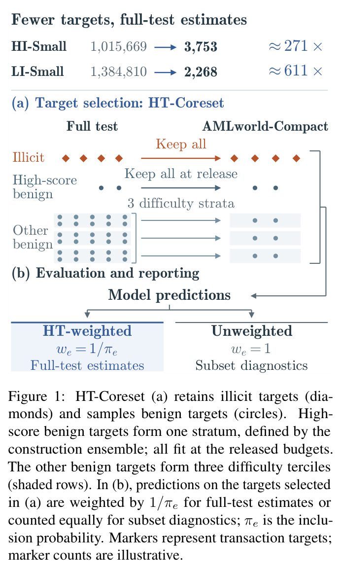
HT-Coreset (a) retains illicit targets (diamonds) and samples benign targets (circles). High-score benign targets form one stratum, defined by the construction ensemble; all fit at the released budgets. The other benign targets form three difficulty terciles (shaded rows). In (b), predictions on the targets selected in (a) are weighted by 1/πe for full-test estimates or counted equally for subset diagnostics; πe is the inclusion probability.
Figure 1: HT-Coreset (a) retains illicit targets (diamonds) and samples benign targets (circles). High-score benign targets form one stratum, defined by the construction ensemble; all fit at the released budgets. The other benign targets form three difficulty terciles (shaded rows). In (b), predictions on the targets selected in (a) are weighted by 1/πe for full-test estimates or counted equally for subset diagnostics; πe is the inclusion probability.
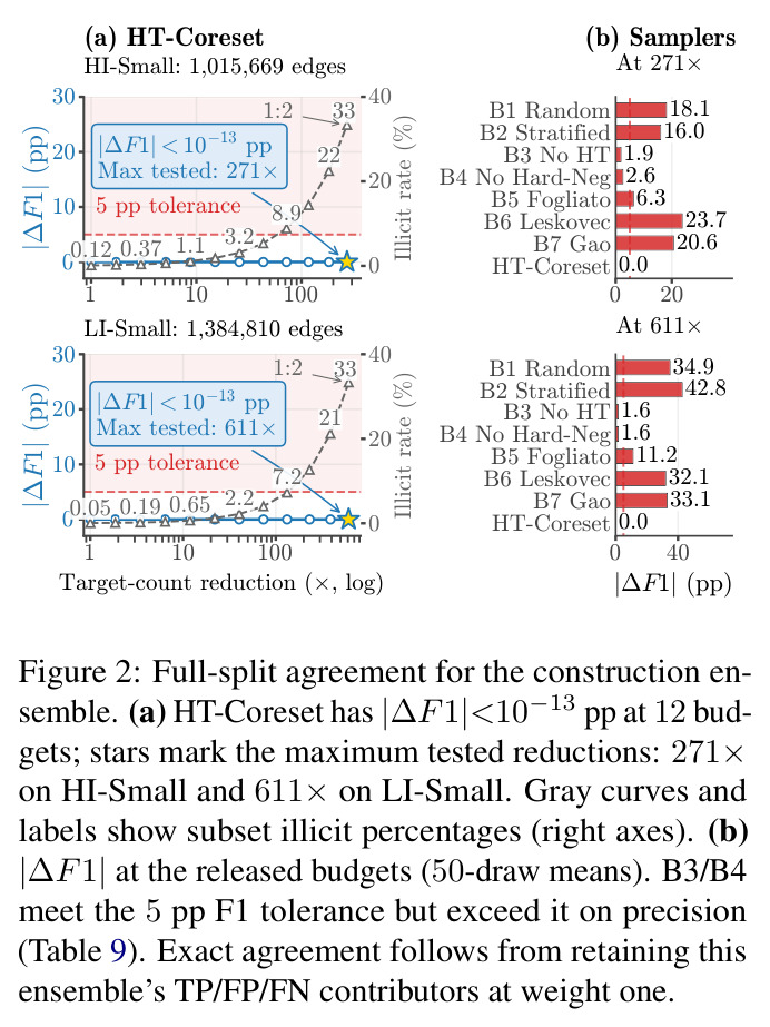
Full-split agreement for the construction ensemble. (a) HT-Coreset has |ΔF1|<10⁻¹³ pp at 12 budgets; stars mark the maximum tested reductions: 271× on HI-Small and 611× on LI-Small. Gray curves and labels show subset illicit percentages (right axes). (b) |ΔF1| at the released budgets (50-draw means). B3/B4 meet the 5 pp F1 tolerance but exceed it on precision (Table 9). Exact agreement follows from retaining this ensemble's TP/FP/FN contributors at weight one.
Figure 2: Full-split agreement for the construction ensemble. (a) HT-Coreset has |ΔF1|<10⁻¹³ pp at 12 budgets; stars mark the maximum tested reductions: 271× on HI-Small and 611× on LI-Small. Gray curves and labels show subset illicit percentages (right axes). (b) |ΔF1| at the released budgets (50-draw means). B3/B4 meet the 5 pp F1 tolerance but exceed it on precision (Table 9). Exact agreement follows from retaining this ensemble's TP/FP/FN contributors at weight one.

实验结果

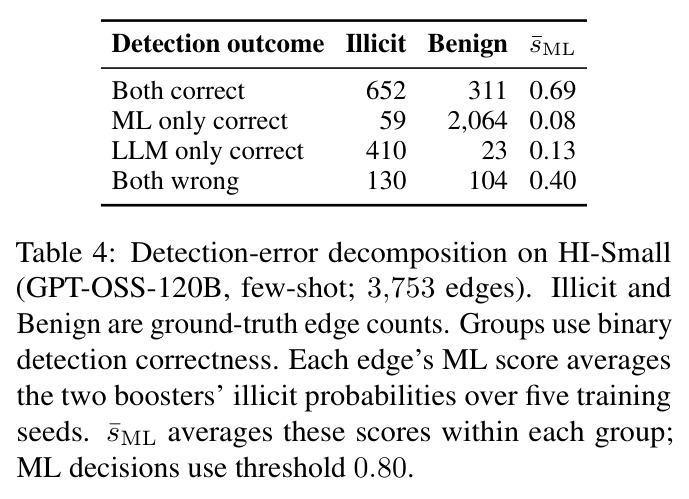
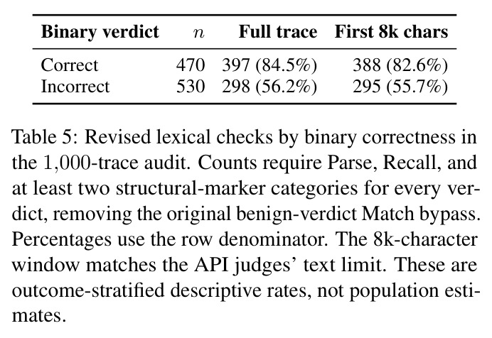
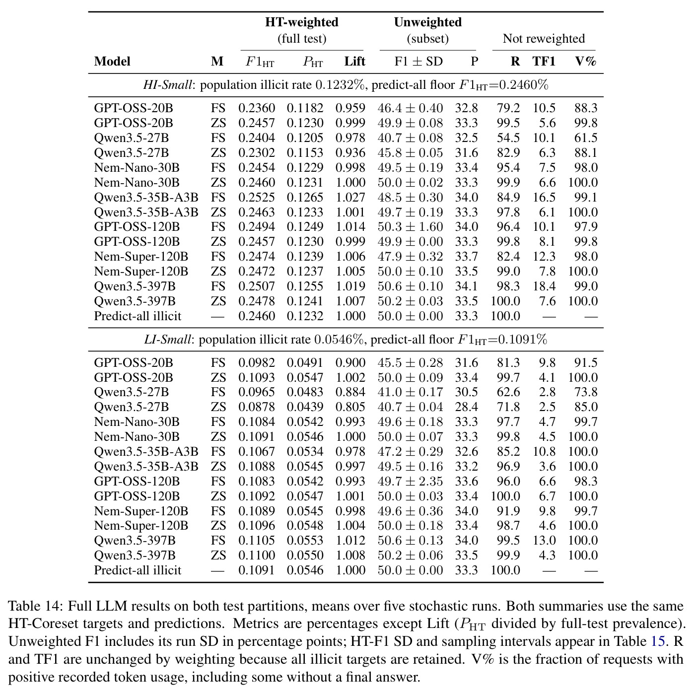
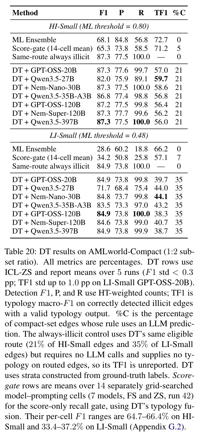
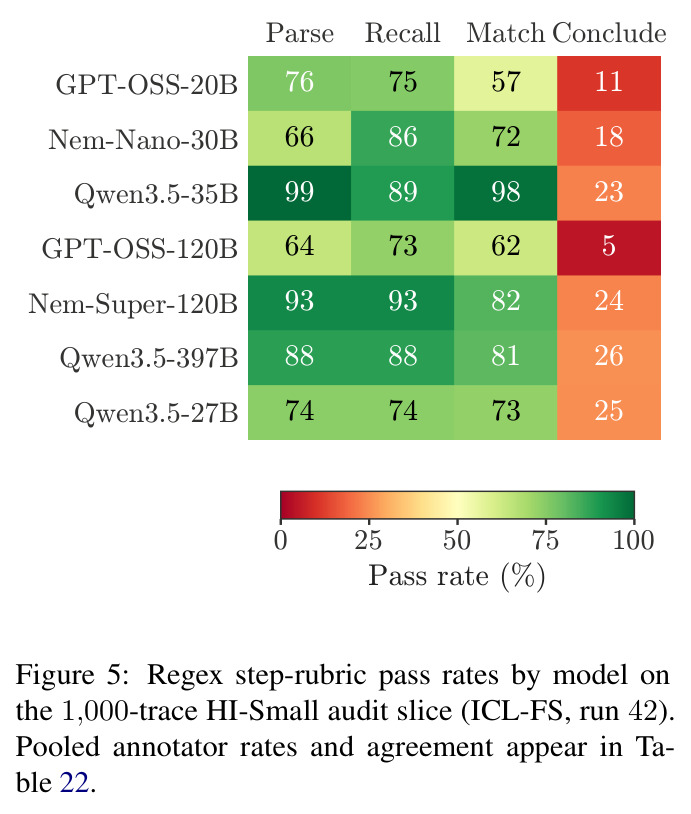
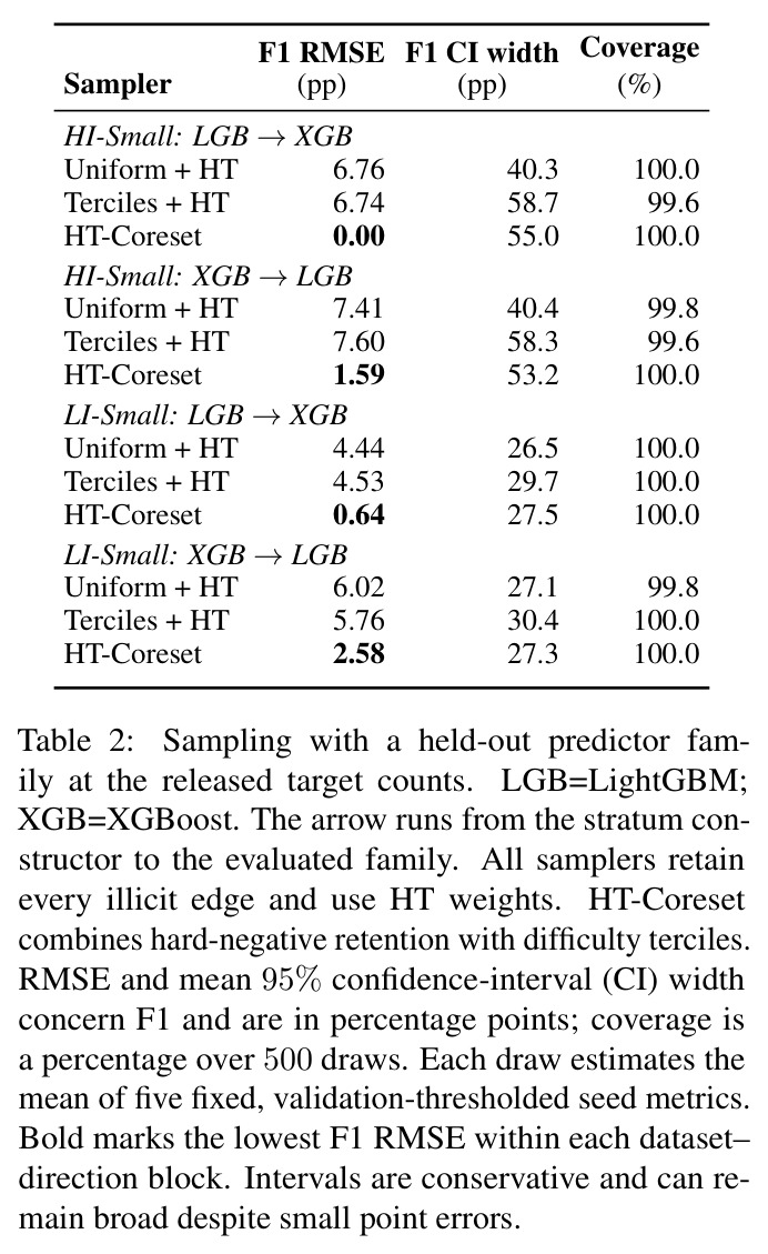
规模与一致性:发布集 3,753(HI,271×)/2,268(LI,611×)个目标,保留全部 1,251/756 条非法边;对参与分层的构造集成,12 个预算下 $|\Delta F_1|<10^{-13}$ pp,P/R 误差精确为 0。held-out 研究(每配置 500 次抽样):发布规模下 HT-Coreset 的 F1 RMSE 为 0.00–2.58 pp,均匀采样+HT 为 4.44–7.41 pp,12 个比较全部最低,但保守区间宽 27.3–55.0 pp。LLM 评估:7 个开源模型的 $F_1^{HT}$ 仅 0.230–0.253%,贴近全预测非法参照 0.246%(lift 0.94–1.03);零样本召回 97.8–100%,高召回无选择性;few-shot 使 7/7 模型 TF1 提升(均值 +5.3 pp),检出无一致变化;$F_1^{HT}$ 在约 5.7× 活跃参数跨度内仅变 0.017 pp。错误重叠:ML-only-correct 2,123 条中 2,064 条为合法(ML 均分 0.08),LLM-only-correct 433 条中 410 条非法(均分 0.13)。trace 审计:词汇检查在正确判定通过 84.5%、错误判定也通过 56.2%。DT 对照:路由 F1 87.3%/84.9% 与同路径全预测非法对照完全一致;Elliptic 上 HT-Coreset 5.1× 压缩精确复现指标,6 个对照显著更差。
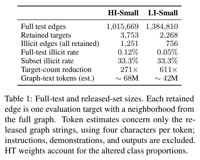
Full-test and released-set sizes. Each retained edge is one evaluation target with a neighborhood from the full graph. Token estimates concern only the released graph strings, using four characters per token; instructions, demonstrations, and outputs are excluded.
Table 1: Full-test and released-set sizes. Each retained edge is one evaluation target with a neighborhood from the full graph. Token estimates concern only the released graph strings, using four characters per token; instructions, demonstrations, and outputs are excluded.
Sampling with a held-out predictor family at the released target counts. LGB=LightGBM; XGB=XGBoost. The arrow runs from the stratum constructor to the evaluated family. All samplers retain every illicit edge and use HT weights. HT-Coreset combines hard-negative retention with difficulty terciles.
Table 2: Sampling with a held-out predictor family at the released target counts. LGB=LightGBM; XGB=XGBoost. The arrow runs from the stratum constructor to the evaluated family. All samplers retain every illicit edge and use HT weights. HT-Coreset combines hard-negative retention with difficulty terciles.
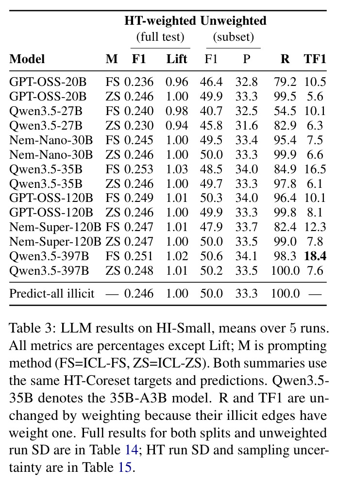
LLM results on HI-Small, means over 5 runs. All metrics are percentages except Lift; M is prompting method (FS=ICL-FS, ZS=ICL-ZS). Both summaries use the same HT-Coreset targets and predictions.
Table 3: LLM results on HI-Small, means over 5 runs. All metrics are percentages except Lift; M is prompting method (FS=ICL-FS, ZS=ICL-ZS). Both summaries use the same HT-Coreset targets and predictions.
Detection-error decomposition on HI-Small (GPT-OSS-120B, few-shot; 3,753 edges). Illicit and Benign are ground-truth edge counts. Groups use binary detection correctness. Each edge's ML score averages the two boosters' illicit probabilities over five training seeds.
Table 4: Detection-error decomposition on HI-Small (GPT-OSS-120B, few-shot; 3,753 edges). Illicit and Benign are ground-truth edge counts. Groups use binary detection correctness. Each edge's ML score averages the two boosters' illicit probabilities over five training seeds.
Revised lexical checks by binary correctness in the 1,000-trace audit. Counts require Parse, Recall, and at least two structural-marker categories for every verdict, removing the original benign-verdict Match bypass. Percentages use the row denominator.
Table 5: Revised lexical checks by binary correctness in the 1,000-trace audit. Counts require Parse, Recall, and at least two structural-marker categories for every verdict, removing the original benign-verdict Match bypass. Percentages use the row denominator.
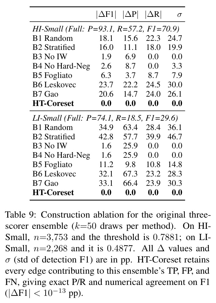
Construction ablation for the original three-scorer ensemble (k=50 draws per method). On HI-Small, n=3,753 and the threshold is 0.7881; on LI-Small, n=2,268 and it is 0.4877. All Δ values and σ (std of detection F1) are in pp.
Table 9: Construction ablation for the original three-scorer ensemble (k=50 draws per method). On HI-Small, n=3,753 and the threshold is 0.7881; on LI-Small, n=2,268 and it is 0.4877. All Δ values and σ (std of detection F1) are in pp.
Supervised detection baselines on the full file-order test partition (mean±std, five training seeds). Means are percentages; stds are in pp.
Table 11: Supervised detection baselines on the full file-order test partition (mean±std, five training seeds). Means are percentages; stds are in pp.
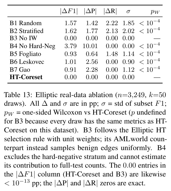
Elliptic real-data ablation (n=3,249, k=50 draws). All Δ and σ are in pp; σ = std of subset F1; pW = one-sided Wilcoxon vs HT-Coreset.
Table 13: Elliptic real-data ablation (n=3,249, k=50 draws). All Δ and σ are in pp; σ = std of subset F1; pW = one-sided Wilcoxon vs HT-Coreset.
Full LLM results on both test partitions, means over five stochastic runs. Metrics are percentages except Lift. R and TF1 are unchanged by weighting because all illicit targets are retained. V% is the fraction of requests with positive recorded token usage.
Table 14: Full LLM results on both test partitions, means over five stochastic runs. Metrics are percentages except Lift. R and TF1 are unchanged by weighting because all illicit targets are retained. V% is the fraction of requests with positive recorded token usage.
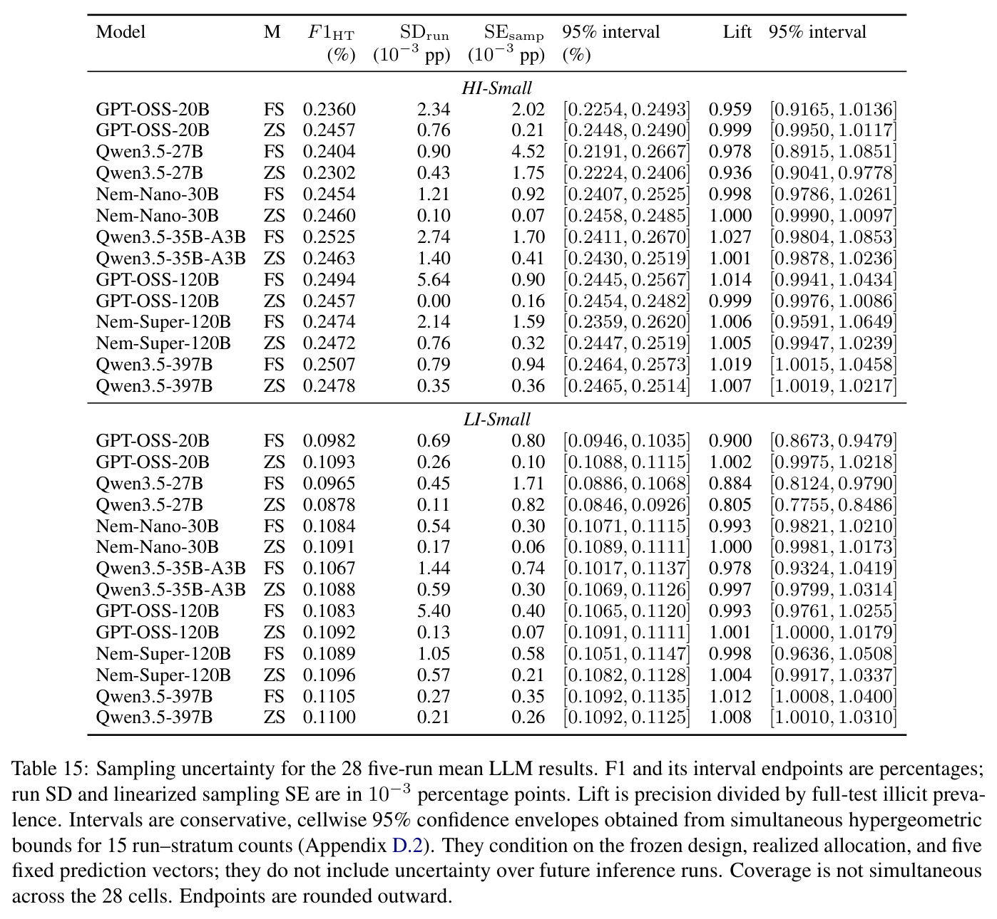
Sampling uncertainty for the 28 five-run mean LLM results. F1 and its interval endpoints are percentages; run SD and linearized sampling SE are in 10⁻³ percentage points. Intervals are conservative, cellwise 95% confidence envelopes.
Table 15: Sampling uncertainty for the 28 five-run mean LLM results. F1 and its interval endpoints are percentages; run SD and linearized sampling SE are in 10⁻³ percentage points. Intervals are conservative, cellwise 95% confidence envelopes.
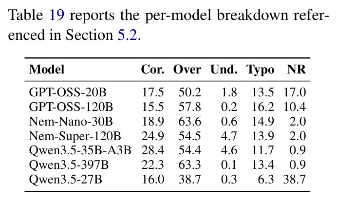
Failure taxonomy on HI-Small (ICL-FS), in percent of cases. Cor.=correct binary verdict and, where a reference exists, correct typology; Over=over-prediction (FP), Und.=under-prediction (FN), Typo=wrong typology given correct detection, NR=no response.
Table 19: Failure taxonomy on HI-Small (ICL-FS), in percent of cases. Cor.=correct binary verdict and, where a reference exists, correct typology; Over=over-prediction (FP), Und.=under-prediction (FN), Typo=wrong typology given correct detection, NR=no response.
DT results on AMLworld-Compact (1:2 subset ratio). All metrics are percentages. DT rows use ICL-ZS and report means over 5 runs. Detection F1, P, and R use HT-weighted counts; TF1 is typology macro-F1 on correctly detected illicit edges.
Table 20: DT results on AMLworld-Compact (1:2 subset ratio). All metrics are percentages. DT rows use ICL-ZS and report means over 5 runs. Detection F1, P, and R use HT-weighted counts; TF1 is typology macro-F1 on correctly detected illicit edges.
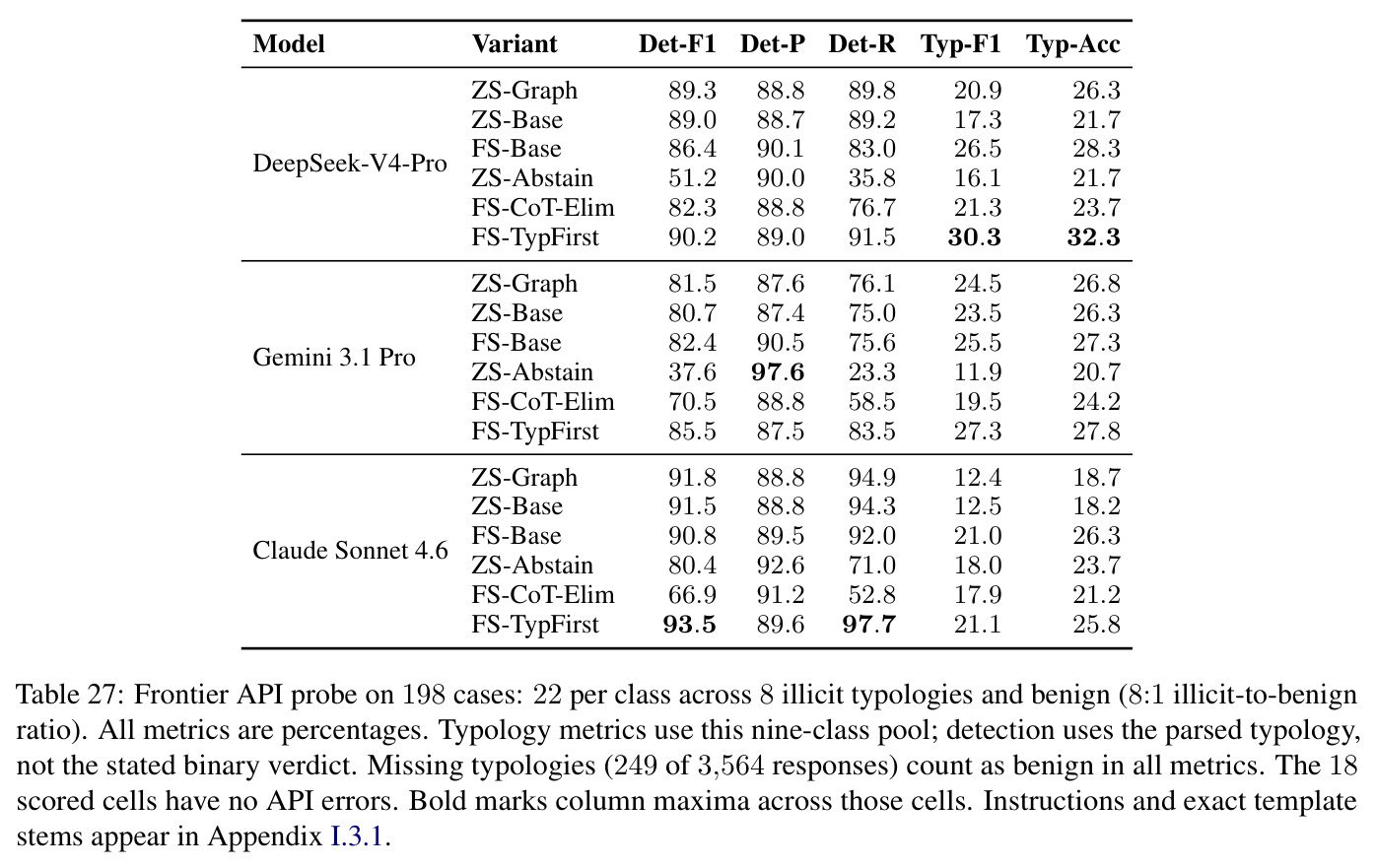
Frontier API probe on 198 cases: 22 per class across 8 illicit typologies and benign (8:1 illicit-to-benign ratio). All metrics are percentages. Typology metrics use this nine-class pool; detection uses the parsed typology, not the stated binary verdict.
Table 27: Frontier API probe on 198 cases: 22 per class across 8 illicit typologies and benign (8:1 illicit-to-benign ratio). All metrics are percentages. Typology metrics use this nine-class pool; detection uses the parsed typology, not the stated binary verdict.
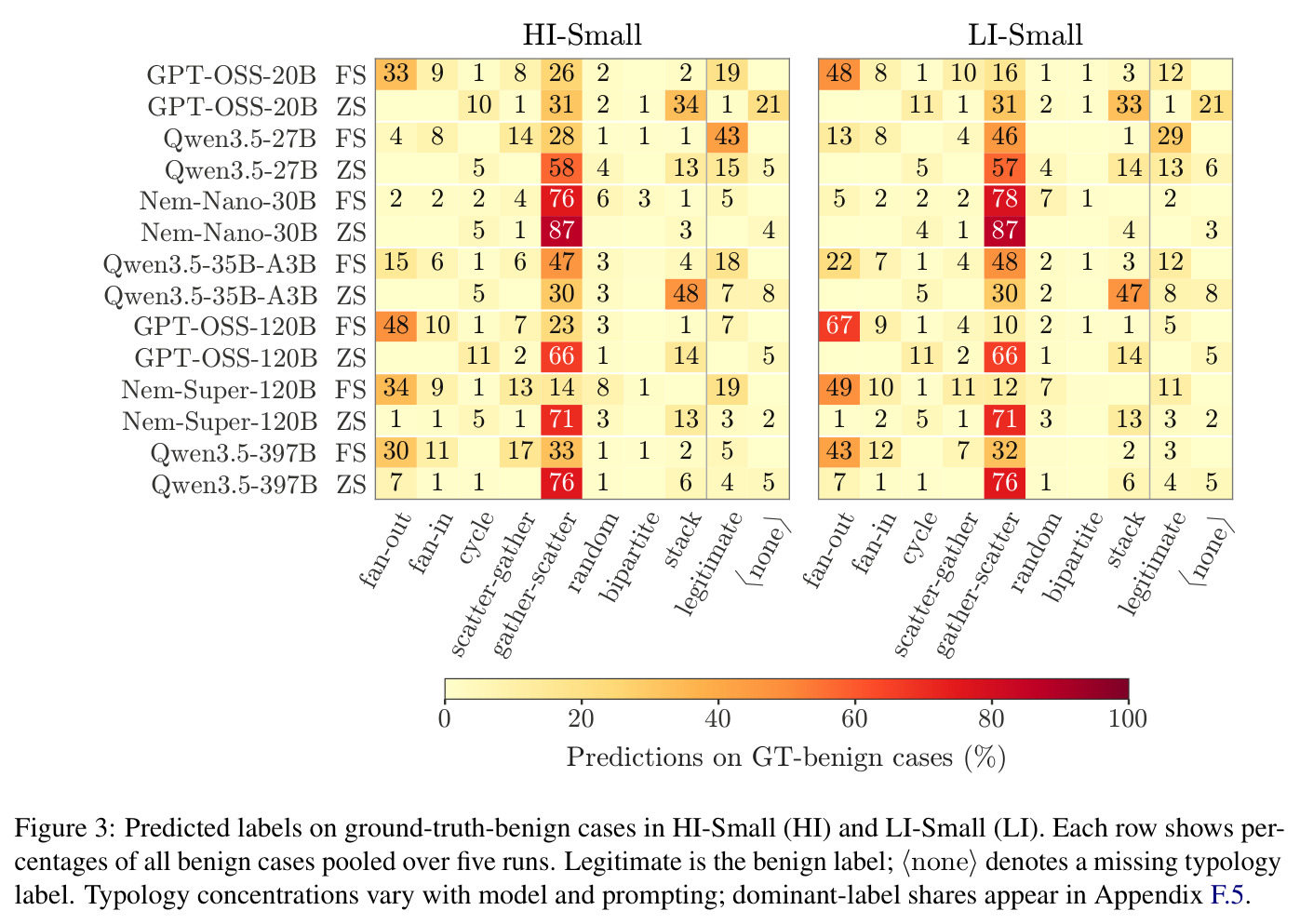
Predicted labels on ground-truth-benign cases in HI-Small (HI) and LI-Small (LI). Each row shows percentages of all benign cases pooled over five runs. Legitimate is the benign label; ⟨none⟩ denotes a missing typology label.
Figure 3: Predicted labels on ground-truth-benign cases in HI-Small (HI) and LI-Small (LI). Each row shows percentages of all benign cases pooled over five runs. Legitimate is the benign label; ⟨none⟩ denotes a missing typology label.
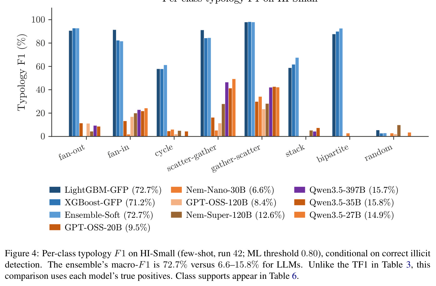
Per-class typology F1 on HI-Small (few-shot, run 42; ML threshold 0.80), conditional on correct illicit detection. The ensemble's macro-F1 is 72.7% versus 6.6–15.8% for LLMs.
Figure 4: Per-class typology F1 on HI-Small (few-shot, run 42; ML threshold 0.80), conditional on correct illicit detection. The ensemble's macro-F1 is 72.7% versus 6.6–15.8% for LLMs.
Regex step-rubric pass rates by model on the 1,000-trace HI-Small audit slice (ICL-FS, run 42).
Figure 5: Regex step-rubric pass rates by model on the 1,000-trace HI-Small audit slice (ICL-FS, run 42).
查看结构化数据
任务指标本文基线提升
全测试 F1 估计(held-out 预测器族,发布规模) F1 RMSE (pp) HT-Coreset 0.00–2.58 均匀采样+HT 4.44–7.41;三分位+HT 4.53–7.60 点误差至少减半,12/12 个数据集×方向×预算比较中最低
评估目标规模 HI-Small 目标数 / 压缩倍数 3,753(271×) 全测试 1,015,669 条边 单次评估成本降约 271 倍
评估目标规模 LI-Small 目标数 / 压缩倍数 2,268(611×) 全测试 1,384,810 条边 单次评估成本降约 611 倍
构造集成的全测试指标复现 |ΔF1| (pp) <10⁻¹³(P/R 精确 0.0) B1 随机采样 18.1(HI)/34.9(LI) 数值级精确一致
LLM 全测试检测(HI-Small,5 run 均值) HT 加权 F1 / 精确率 lift 0.230–0.253% / lift 0.94–1.03 全预测非法参照 0.246% / 1.00 基本持平——原始图 prompt 下 LLM 无实质判别力
类型学识别(HI-Small few-shot) TF1 (%) 18.4(Qwen3.5-397B) 同模型零样本 7.6 +10.7 pp;7/7 模型提升,均值 +5.3 pp
ML 参照 vs LLM 子集检测(HI-Small) 检测 F1 (%) ML 双 booster 集成 68.1(全测试) LLM 无加权子集 F1 最高 50.6 ML 领先约 17.5 pp,LLM 未达监督基线
Elliptic 真实数据外部校验 |ΔF1| 均值 (pp) HT-Coreset 0.00(5.1× 压缩) 6 个对照 0.91–3.79(B4 的 |ΔP| 达 10.01) Wilcoxon p<10⁻⁴,显著最低

局限与改进

作者承认的局限:主评估仅覆盖 7 个开源权重模型、两个最小合成切分与单一图-文本管线,对更大图和真实银行数据的泛化未验证;原始输入不标记目标交易——324/3,753(HI)与 297/2,268(LI)的上下文中目标完全缺席,其余案例也只留 占位符,错误无法完全归因于模型推理;CSV 顺序划分时间戳重叠,非严格前瞻;ML 参照与 DT 的阈值在全测试标签上选出,属探索性比较;采样不确定性基于冻结设计与 5 个固定预测向量,未经全测试 LLM 预测或独立核心集抽样检验;保守区间宽达 27–55 pp,点估计改进不等于精确估计。我的补充:GCPAL 复现的微调划分与测试集约 60% 重叠,只能留在冻结构造中;精确性只对构造集成成立,GCPAL 偏差 3.9 pp、LI 上 XGB→LGB 的 P RMSE 达 9.7–10.2 pp,对无关预测器的迁移仍开放;Qwen3.5-27B 因 128K 部署上限出现 38.7% 无响应;人工 trace 审计仅 28 条记录且 Match 一致性 κ=0.10,API judge 也看不到交易图。

独立分析的弱点

独立分析出的弱点:第一,对监督分层的依赖是结构性风险——精确性论证只覆盖构造集成,被评估模型若在保留的难负层之外标记合法边(如 GCPAL |ΔF1| 3.9 pp,LI 的 XGB→LGB P RMSE 10.2 pp),估计就会失准;改进方向是用多个异构模型族建层,并给出对任意预测器的稳健误差界。第二,置信区间太宽(27–55 pp),实际上无法在模型间做等价性或优劣判断;可引入配对线性化标准误、序贯抽样或更紧的方差估计。第三,输入缺陷未修复就下结论:目标缺席/不标记意味着'高召回'可能只是对整图的粗略怀疑,作者发布了 target-marked 版本却未做配对评估,应补上以定位真实推理能力。第四,1:2 富集使无加权 F1(约 50%)与 HT F1(约 0.25%)相差约 200 倍,双口径极易被误读,报告模板应更显式地绑定口径。第五,全部实验在合成数据上进行,frontier probe 显示最强模型的类型学宏 F1 也仅 30.3%,且 56.2% 的错误判定也通过词汇检查,提示'会说洗钱术语'不等于'有图证据支撑',正确率与解释质量脱钩。

未来方向

作者提出的方向:在配对设计中评估 target-marked 输入对预测的敏感性(当前只做了完整性与序列化检查);把协议推广到更大的 AMLworld 切分与真实交易图,新图需重建分层并入样概率;把采样不确定性检验扩展到全测试 LLM 预测与独立核心集抽样。基于本文成果可延伸的:一是自适应/序贯抽样,在同等预算下收窄目前 27–55 pp 的宽区间;二是研究不依赖标签分层的 ML–LLM 路由——DT 的收益几乎全部来自标签分层的路径本身,score-only 门控在 LI 上 F1 仅 34.2%,说明可部署的混合推理仍是开放问题;三是改进类型学识别(few-shot 收益 +5.3 pp、frontier probe 的 FS-TypFirst 也只到 30.3%),把结构-类型学推理作为专门评测维度;四是把'词汇检查 vs 图证据支撑'的差距发展成 faithfulness 评估,结合不忠实解释文献(Turpin 等)设计配对探针;五是检查 AML 类型学词表可能带来的提示泄露/数据污染对结论的影响。

复现评估

复现条件好、门槛中等。开源:评估集在 HuggingFace(typhoon-ai/AMLworldCompactEval),GitHub(nat-nischw/AMLworld-Compact)提供建构代码、审计工具、target-marked prompts、逐抽样/逐 seed CSV、输入哈希与验证报告;代码、ML 参数与全测试模型输出为 MIT,数据集为 CDLA-Sharing;Elliptic 因 CC BY-NC-ND 仅发布代码,SLURM 脚本在 16 核 CPU 约 1–2 小时复现全部数字。算力:目标选择用 seed 0 可从构造分数精确复现;GFP booster 训练约 3 H100-小时;LLM 推理用 vLLM 于 H100/H200 共约 2,840 GPU 小时(Qwen3.5-397B 约 1,320),共 433,512 次请求、24.91B 输入 + 0.90B 输出 token。难点在 LLM 部分:多卡集群、上下文部署(Qwen3.5-27B 因 128K 上限产生 38.7% 无响应)与推理工程;采样/ML/Elliptic 管线普通工作站即可。

相似论文推荐