Fathom:面向卸载 KV 缓存稀疏解码的逐查询读取深度 Fathom: Per-Query Read Depth for Sparse Decoding over Offloaded KV Caches
4位K缓存按位平面存储,查询逐通道逆注水分配读取位深,主机内存索引解码步最高提速1.67倍
前置知识
KV 缓存与解码带宽瓶颈
自回归生成时,每个已生成 token 的 key/value 向量都要被缓存;生成长上下文时,每步解码要把全部历史 KV 读一遍。小模型(如 8B 级)每步读权重的开销相对固定,而 KV 读取随上下文长度线性增长,因此长上下文解码是带宽受限问题:每步时间由跨内存层级搬运的数据量决定,而不是由算力决定。
论文测量的正是这一步的流量构成:当 KV 缓存与其排名索引驻留主机内存时,扫描字节成为瓶颈。理解“少读几个比特”为何能直接换算成加速,必须先建立这个带宽瓶颈模型。
Top-k 稀疏注意力与扫描—选择两步
注意力质量集中于少数 key,所以解码时先用一个便宜的表示给全部 n 个 key 打近似分,选出每查询头的 top-k,再只取这些行的完整 K/V 做精确注意力。打分阶段要读全部 n 条压缩记录,字节量随上下文线性增长;取回胜者行的代价却不随上下文增长。
Fathom 优化的正是第一步“扫描”的字节数;Loki、Double Sparsity、SparQ、缩略图扫描等基线都是这一两步框架的不同实例,全文的对比协议也建立在此框架上。
KV 缓存卸载(offloading)与 PCIe
多会话长上下文使 KV 缓存放不进 GPU 显存时,缓存保存在主机内存等更慢层级,每步通过 PCIe(本文平台上约 26 GB/s)搬运。此时步时间近似等于字节数除以链路速率,节省字节几乎线性转化为节省时间;而数据全在 HBM 时这个等价关系不成立。
论文全部时间收益都在这一机制下测得;作者也诚实指出索引驻留 HBM 时方法不再更快。理解该前提是判断方法适用范围的关键。
GQA(分组查询注意力)
多个查询头共享一个 KV 头:Qwen3-8B 有 8 个 KV 头、每头 128 个通道,每 4 个查询头共享 1 个 KV 头,共 288 个“层–KV头”对。同一组的查询头只需一份扫描:聚合组内查询的打分来选通道或选胜者行,K 字节只读一次供全组使用。
Fathom 的通道重要性 $g_j$ 与读取计划都按 KV 头组计算;全文的比特约定(每 token 每 KV 头每层)也建立在这一结构之上。
均匀标量量化与位平面
把每通道数值用对称均匀码量化为 4 比特整数,外加每 64-token 块一个 fp16 缩放因子。将各码字按位分层、通道主序存储后,任一通道的前 $t$ 个位平面恰好构成该通道的 $t$ 比特均匀量化器:前缀读取无需另存低精度副本就是精确的更粗量化。非均匀码(如 Lloyd–Max、查表码)没有这个性质。
这是全文的存储基石:只有“前缀 = 精确低精度量化器”才能让读取深度成为运行时逐查询决策,而不需要维护多套精度副本。
逆注水(reverse water-filling)位分配
率失真理论中的经典最优比特分配策略:当各通道误差按每比特 4 倍速度衰减时,边际收益最大的通道先拿比特,其余通道的深度由自身重要性与公共水位线 $\theta$ 之差的对数给出,在总预算约束下可通过对数二分求得闭式解。
Fathom 把“这个查询该对每个通道读几位”形式化为预算 $B$ 下的注水分配,这是方法的数学核心,也是与所有固定深度扫描的本质区别。
研究动机
编码或浏览智能体会话持续数小时、上下文达数十万 token,服务器同时驻留多个会话,KV 缓存放不进显存而驻留主机内存,每步解码受互连带宽限制。以 Qwen3-8B(36 层、8 个 KV 头×128 通道、每 KV 头 4 个查询头)在 32k 上下文为例:稠密 bf16 注意力每步读 4.8 GB KV;k=512 的 top-k 稀疏注意力只需取回约 200 MB 胜者行且不随上下文增长,但给全部 key 排名的扫描要读 136 bit/token(Loki、Double Sparsity、SparQ r=32 的统一字节数),288 个层–KV头对合计每步约 160 MB,线性增长到 1M token 时的 5.1 GB——扫描而非取行成为瓶颈。现有逐 token 扫描方法各有通道选择策略:Loki 读 32 个 PCA 主成分坐标,Double Sparsity 读离线选定的 32 个通道,SparQ 让查询选组内 $|q_j|$ 最大的 16 或 32 个通道,缩略图扫描则全通道读 2 bit;但它们被触及的每个通道的读取深度都是设计期固定的,与具体查询无关,大量字节浪费在该查询根本不依赖的通道上。
本文的目标是本文的目标是:在保住 top-k 排名精度的前提下,把每步扫描字节数压到固定深度扫描之下,并在“KV 缓存与索引驻留主机内存”的目标场景中把字节节省转化为 GPU 时间节省;同时存储本身应当就是量化服务栈已有的那份 4 比特 K 副本(68 B/token/KV头),不引入额外索引结构。可量化的目标包括:在等 GPU 时间内比 SparQ r=16(68 bit)读更少字节且注意力误差更低;达到 Double Sparsity 或 SparQ r=32(均 136 bit)的误差时读取位数减半以上;在 RULER 风格检索任务上与精确 top-k oracle 打平;在真实编码智能体会话上,逐步一致性(step agreement)超过同字节的 SparQ r=16;并且明确给出方法失效的边界条件——索引驻留 HBM 时不再更快。
与已有工作不同的是,本文的独特切入是把两个此前未被组合的观察结合起来。其一,均匀量化器每多读 1 bit,通道对得分的剩余误差方差按 4 倍衰减,因此不同通道、不同深度的第 N 个比特边际价值差异巨大:重要通道的第一比特可能比次要通道的第四比特还值钱,最优分配正是经典逆注水。其二,若把 4 比特 K 缓存按通道主序存成位平面,前缀读取天然就是精确的 $t$ 比特量化器,块缩放不变、无需低精度副本。两者结合把“读取深度”从设计期常量变成每个查询、每个通道的运行时决策。这一杠杆与“少打分对象”的块/地标方法(Quest、ShadowKV、InfLLM)正交;与把压缩 K 当索引的 Self-Indexing KVCache、FFD 相比,差异正在于深度可变。作者还补上了同类工作中少见的诚实分析:用每字节算术量解释为何索引在 HBM 时方法不更快,并给出字节比何时近似时间比的判据。
核心方法
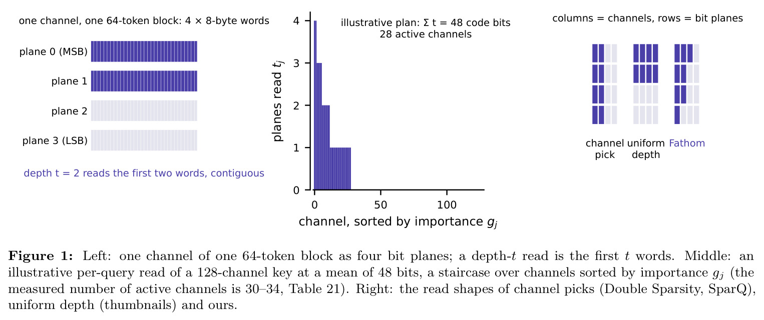
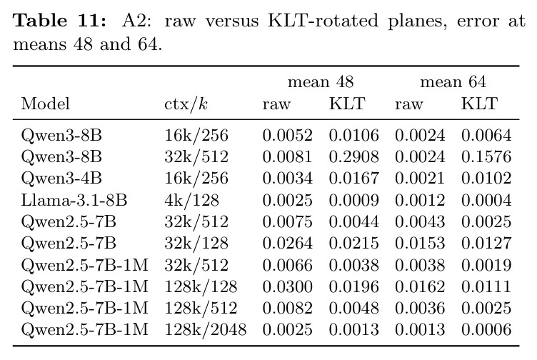
直觉:一个查询真正依赖的通道极少且深浅需求不一——重要通道的前几个比特价值远高于末位比特,次要通道一比特都不值得读。技术路线分两半。存储侧:把 K 量化为 4 bit 均匀对称码、每 64-token 块一个 fp16 缩放(式 2),按通道主序打包成位平面,前 $t$ 个平面的反量化值恰是 $t$-bit 中升量化器。计算侧:解码时对共享同一 KV 头的查询组计算各通道得分方差贡献 $g_j=\sum_h (q_j^{(h)})^2\,\mathrm{Var}(k_j)$(式 3),在预算 $\sum_j t_j \le B$ 下按 $t_j=\mathrm{clip}(\mathrm{round}(\log_4(g_j/\theta)),0,4)$ 逆注水分配深度(式 4),30 步对数二分求水位线 $\theta$。读取时 gather kernel 按“每活动通道一段 $t_j n/8$ 连续字节”从 pinned 主机内存以约 26 GB/s 搬入 HBM,再在 HBM 内完成扫描与逐查询头 top-k,最后取胜者行做精确注意力。基准规则:有 QK-norm 的模型(Qwen3)用原始通道,无 QK-norm 的(Llama-3.1、Qwen2.5)用 KLT 旋转平面。
核心创新有二。其一,位平面存储使“前缀读取 = 精确低精度量化器”:因为码是均匀的,通道前 $t$ 个平面的反量化值恰是区间 $[-a_{\beta,j}, a_{\beta,j})$ 上的 $t$-bit 中升量化器,块缩放不变,任意深度前缀都无需校正或多副本——这是 Any-Precision LLM 用于权重的位平面思想,首次以“逐查询、逐通道前缀”的方式用于 K 缓存扫描,存储即索引且分辨率可变。其二,读取深度由逆注水在线决定:第 $t_j+1$ 个比特对该查询得分误差的边际收益按 $g_j 4^{-t_j}$ 衰减,注水把比特集中到该查询真正依赖的通道上。与已有方法的本质区别在于:Loki 与 Double Sparsity 的通道离线固定,SparQ 按 $|q_j|$ 排名对 r 个通道全有全无,缩略图全通道均匀 2 bit——四者的读取深度都不随查询变化;Fathom 的读取计划按 KV 头组共享、K 字节只读一次,深度梯度化,且重要性 $g_j$ 用键方差加权而非只看查询幅值,理论上在等字节下误差更低。
方法步骤详情
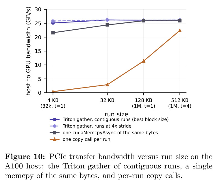
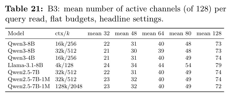
流程五步。(1) 离线:在 Wikitext-103 校准每通道键方差与(无 QK-norm 模型的)KLT 特征基;把全层 K 量化为 4 bit、通道主序位平面加 fp16 块缩放;无 QK-norm 模型存 $(k-\mu)V$ 的平面并按得分方差排序特征,$g_j=\sum_h ((q^{(h)}V)_j)^2\lambda_j$。(2) 逐步计划:对每个 KV 头的查询组算 $g_j$,按式 4 以 30 步对数二分求最小可行水位线 $\theta$,得到各通道深度 $t_j\in[0,4]$ 与活动通道集(预算 48 时约 30–34 个)。(3) 传输:Triton gather kernel 以固定 run list(每活动通道一槽,槽长 $t_j n/8$ 字节)把各通道前 $t_j$ 平面的连续段与缩放拷入 HBM 暂存区,无主机同步,实测 25.1–26.2 GB/s,与单次 memcpy 同速。(4) 扫描与选择:在 HBM 内反量化已读平面、对 n 个 key 打近似分,按查询头独立取 top-k。(5) 取行与精确注意力:经 PCIe 取回组内并集胜者行的 bf16 K/V 做精确注意力。可选逐层贪心预算 $B_\ell\in[24,128]$,但默认推荐平预算。
技术新颖性
技术新颖性体现在五点。(1) 存储即索引且分辨率可变:位平面 K 缓存同时是服务栈的 K 副本和多分辨率索引,前缀读取无信息损失,区别于 Loki(PCA 截断副本)、Double Sparsity(17 B/token 标签缓存)、SparQ(fp16 通道主序存储)等“另建一份索引”的路线。(2) 深度在线化:把率失真论的逆注水用于注意力扫描的逐查询位分配,给出闭式解与 30 步对分实现,将读取深度从设计期常量变成运行时函数。(3) 对量化家族的兼容性分析严谨:均匀整型码(含 KIVI 通道码、INT8)直接可用;非均匀码、KVQuant 查表码、Lloyd–Max 不可用;量化前旋转须集中方差(KLT 可用)而非摊平方差(TurboQuant 的随机旋转不可用)。(4) 罕见的负结果分析:以每字节整型算术量(A100 约 5 ops/byte)与 Amdahl 定律解释索引驻留 HBM 时为何无加速,并给出“PCIe 上字节比趋近时间比”的判据。(5) 逐层预算、基准选择规则(QK-norm→raw 平面,否则 KLT 平面)均由跨模型测量决定而非假设。
实验结果
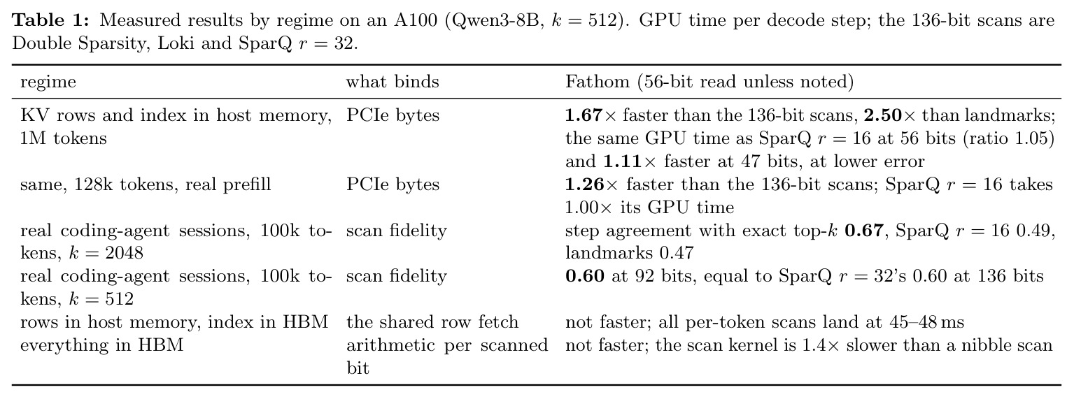
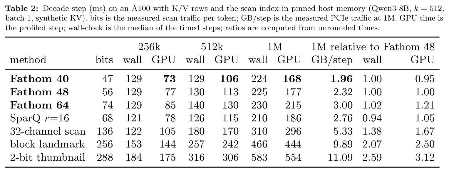
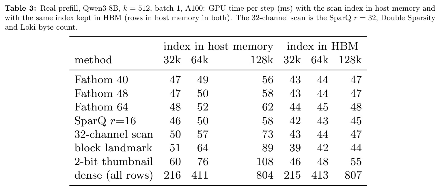
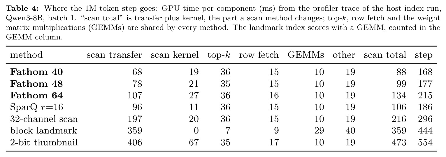
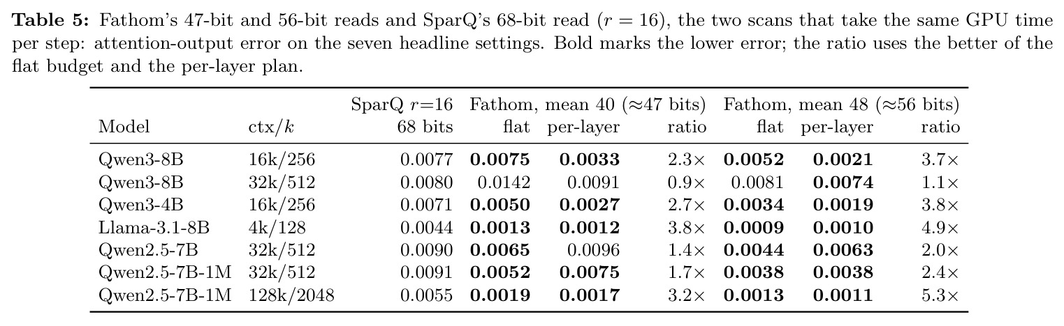
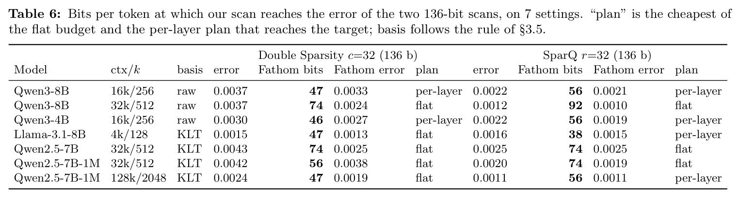
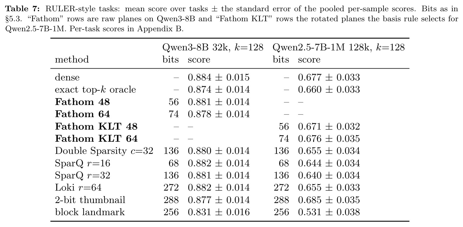
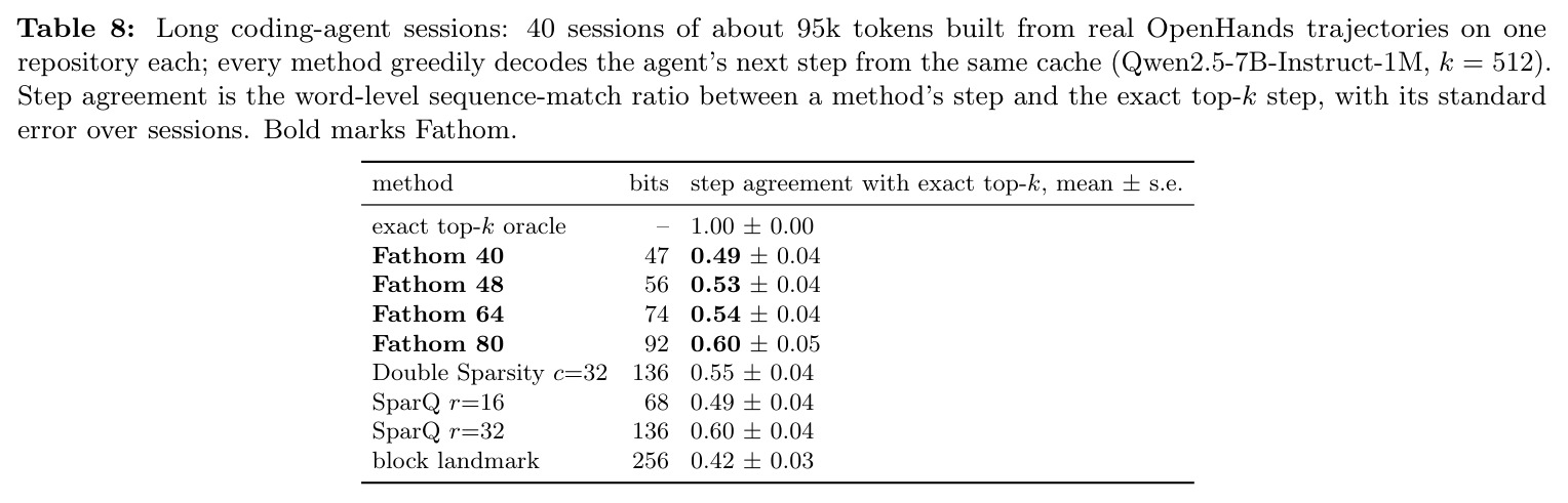
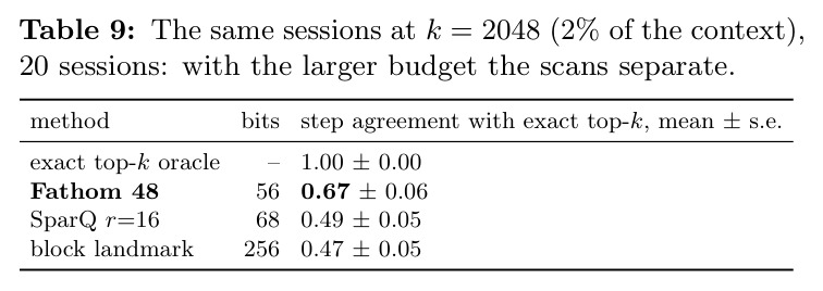
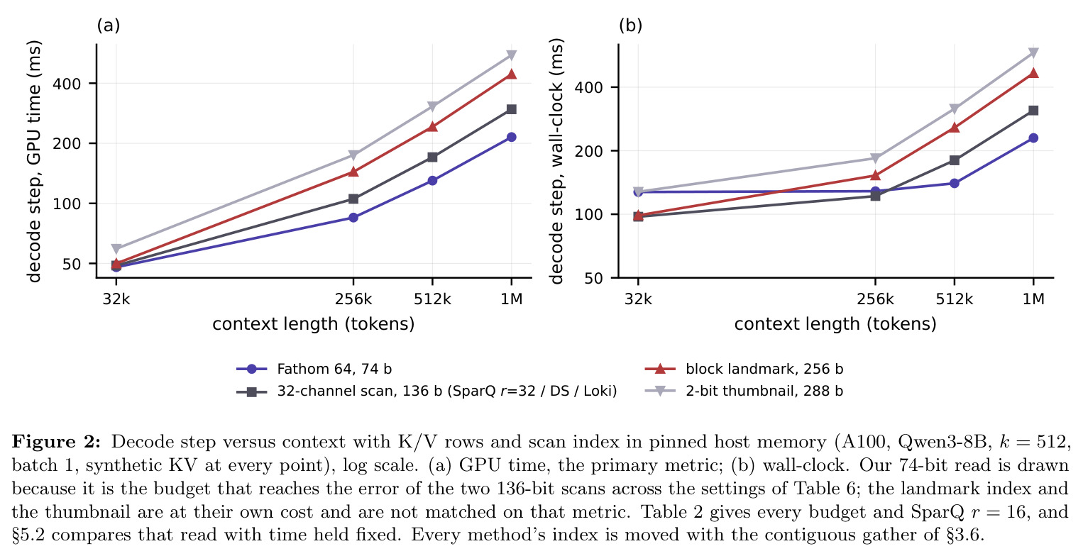
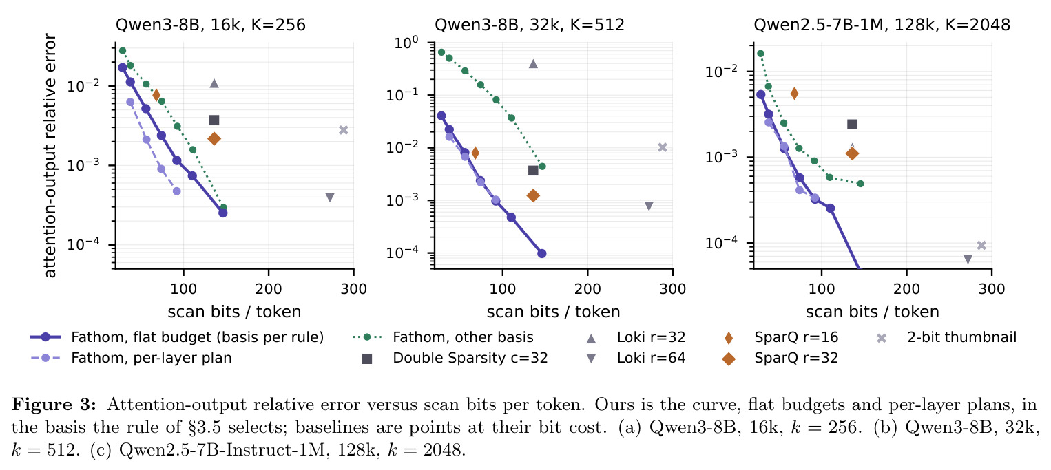
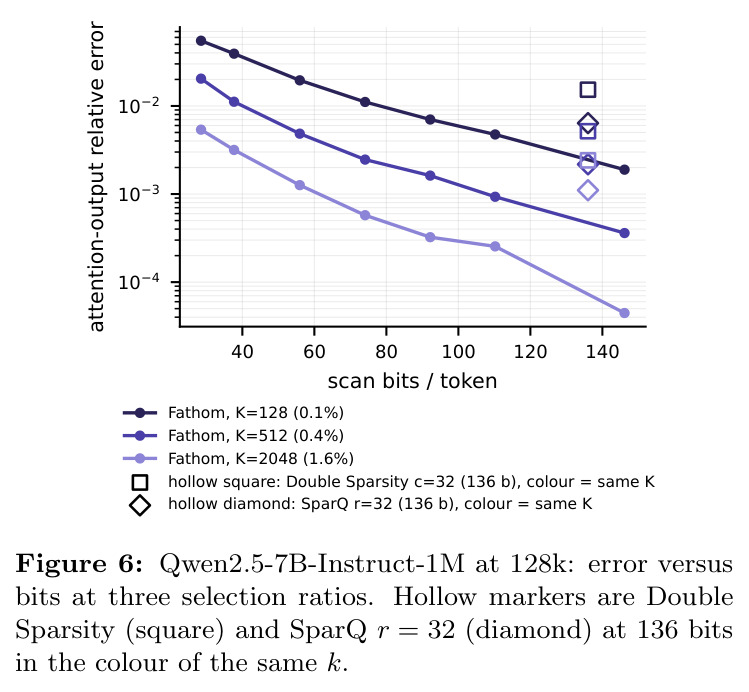
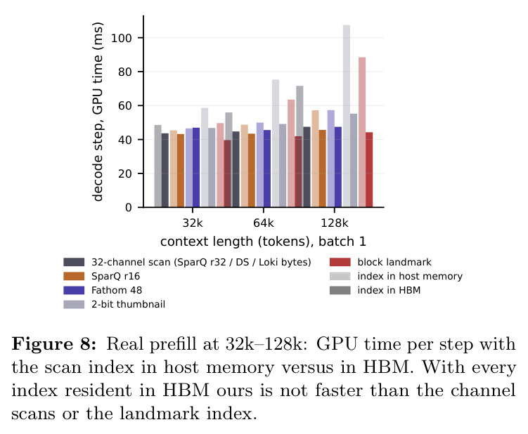
目标场景:索引驻留主机内存(A100,Qwen3-8B,k=512)。1M 上下文时 Fathom 48(56 bit)GPU 时间/步 177 ms,比 136 bit 三扫描(296 ms)快 1.67×、比块地标快 2.50×、比 2-bit 缩略图快 3.12×;47 bit 读取比 SparQ r=16 快 1.11×(少 31% 字节);56 bit 打平(1.05×)但少 22% 字节。等时间下比 SparQ r=16 少读 18% 字节、注意力误差低 1.1–5.3×(7/7 设置);等误差下达到 Double Sparsity(136 bit)只需 46–74 bit(省 1.8–2.9×),达 SparQ r=32 需 38–92 bit。RULER 上各扫描与 oracle 差距小于一个标准误(Fathom 0.881 对 0.874),块地标掉 0.043。真实 OpenHands 会话(约 95k token):k=2048 时 Fathom 48 一致性 0.67±0.06,对 SparQ r=16 的 0.49 配对 +0.18±0.05;k=512 时最强基线 SparQ r=32 为 0.60,Fathom 80(92 bit)少 32% 字节打平,56 bit 的 0.53 高于 SparQ r=16 的 0.49。
查看结构化数据
| 任务 | 指标 | 本文 | 基线 | 提升 |
|---|---|---|---|---|
| 主机内存索引下的 1M-token 解码步(Qwen3-8B,k=512,A100,batch 1,合成 KV) | GPU 时间/步 | Fathom 48(56 bit)177 ms;Fathom 40(47 bit)168 ms | 136-bit 扫描(SparQ r=32 / Double Sparsity / Loki)296 ms | 1.67×(56 bit)/ 1.77×(47 bit) |
| 同场景,与弱基线对比 | GPU 时间/步 | Fathom 48:177 ms | 块地标(256 bit)444 ms;2-bit 缩略图(288 bit)554 ms | 2.50×(地标)/ 3.12×(缩略图) |
| 等 GPU 时间的精度对比(7 个模型/上下文设置) | 注意力输出相对 L2 误差 | Fathom 56 bit,少读 18% 扫描字节,误差低 1.1–5.3×(最佳配比 7/7,平预算 6/7) | SparQ r=16(68 bit),GPU 时间为其 1.05×(1M)/1.00×(128k) | 47 bit 读取还快 1.11× 且 6/7 设置误差更低 |
| 达到 136-bit 扫描精度所需的读取位数(7 设置) | 扫描 bit/token(等误差) | 达 Double Sparsity 误差需 46–74 bit;达 SparQ r=32 需 38–92 bit | Double Sparsity 与 SparQ r=32 均为 136 bit | 对 DS 字节节省 1.8–2.9×;对最强基线 SparQ r=32 最高省 3.6× |
| RULER 风格任务,Qwen3-8B 32k,k=128(6 任务×40 样本) | 金串命中率(mean ± s.e.) | Fathom 48(56 bit)0.881 ± 0.014 | 精确 top-k oracle 0.874 ± 0.014;稠密 0.884 ± 0.015;块地标 0.831 ± 0.016 | 与 oracle/稠密打平(差距小于标准误),超地标约 +0.05 |
| RULER 风格任务,Qwen2.5-7B-1M 128k,k=128 | 金串命中率 | Fathom KLT 64(74 bit)0.676 ± 0.035 | oracle 0.660 ± 0.033;SparQ r=16(68 bit)0.644;块地标 0.531 | 超过 oracle,超 SparQ r=16 约 +0.032 |
| 真实 OpenHands 编码会话(约 95k token,20 会话,k=2048 即 2% 预算) | 与精确 top-k 步骤的逐步一致性 | Fathom 48(56 bit)0.67 ± 0.06 | SparQ r=16(68 bit)0.49 ± 0.05;块地标(256 bit)0.47 ± 0.05 | 对 SparQ r=16 配对 +0.18 ± 0.05(14/20 会话),字节少 18%、GPU 时间相同 |
| 真实编码会话(40 会话,k=512 即 0.5% 预算) | 逐步一致性 | Fathom 80(92 bit)0.60 ± 0.05 | SparQ r=32(136 bit)0.60 ± 0.04(最强基线);SparQ r=16 0.49;DS 0.55 | 以少 32% 字节打平最强基线;56/74 bit 的 0.53/0.54 也高于 SparQ r=16 |
| 对照实验:索引驻留 HBM(真实 prefill,128k,Qwen3-8B) | GPU 时间/步 | Fathom 48:47 ms | 32 通道扫描 47 ms;块地标 44 ms;缩略图 55 ms | 无加速:所有逐 token 扫描落在 45–48 ms(方法的前提是索引在慢层) |
局限与改进
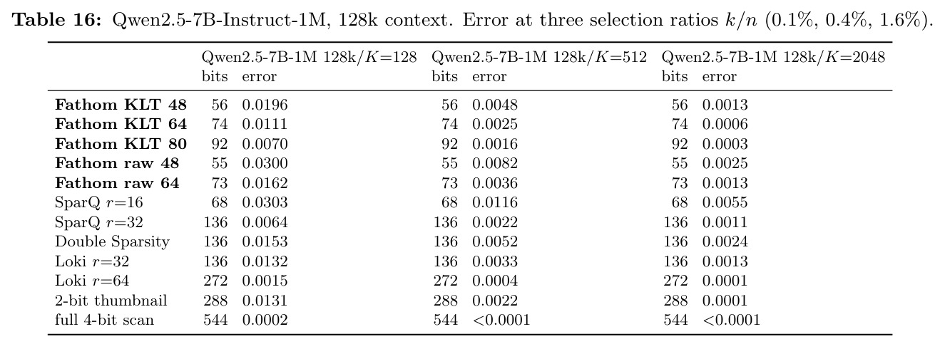
作者承认的局限:方法只在索引驻留慢层时更快,索引在 HBM 时与 4-bit 通道扫描持平(45–48 ms);独立索引存储 68 B/token/KV头,是 DS 标签缓存(17 B)的 4 倍、地标(32 B)的 2 倍,只有 K 缓存本就 4-bit 通道主序的服务栈才免费;质量只在注意力误差、合成 RULER 任务与 40/100 个会话的 step agreement 上测量,端到端带测试执行的任务成功率未测;RULER 对该量级扫描误差不敏感;地标基线是 ShadowKV 块均值的重实现,未与 RetroInfer/MagicPIG 类 CPU 检索比较;128k 以上计时用合成 KV;batch 1 为主,多会话场景由索引体积推断而非实测。我的补充:收益绑死 PCIe 链路速率与主机内存品质,换平台比例会变;per-layer 校准跨模型忽好忽坏(Qwen3 16k 误差减半,Qwen2.5/Llama 恶化至 1.7–2.1×)、跨上下文不可迁移;误差随选择率 $k/n$ 缩小而放大,0.1% 时对 SparQ r=16 优势从 4.4× 收窄到 1.6×,小 k 超长上下文是软肋;通道主序布局按 token 重构单个 key 不便宜,与需要随机访问单条 KV 的应用有摩擦。
独立分析的弱点
独立分析的弱点与改进方向:(1) 扫描 kernel 算术受限——位平面 kernel 每提取 1 bit 需移位掩码加 G 次乘加,HBM 内带宽仅为 nibble 扫描的 1/3–1/2,即便在 PCIe 上与 SparQ r=16 也只打平;改进方向是按 $t_j$ 编译期特化 kernel、把相邻 token 同位打包成宽字提取、或设计位平面专用 SIMD/Tensor Core 路径。(2) 存储放大——独立索引 68 B/token 显著推高内存预算;改进方向是论文指出但未实现的“平面即 K 缓存”服务栈:胜者行直接由四平面重构,消掉独立索引。(3) 小选择率下误差放大(15× 对固定深度的 5–6×);改进方向是让总预算 $B$ 随 $k/n$ 自适应,或在低信噪比层自动升级读取深度。(4) per-layer 离线校准跨模型不稳定、跨上下文长度不可迁移(16k 校准用于 32k 反而更差);改进方向是用层内在线误差反馈做运行时预算调节。(5) 兼容面窄——非均匀码、KVQuant 查表、向量量化都不适用;改进方向是为残差 VQ 的分级结构设计逐级前缀读取,把可变深度推广到更多量化家族。
未来方向
作者提出的方向:端到端带测试执行的真实智能体任务评估(现止步于 step agreement);融合实现消除 research harness 的每方法 Python 开销;与 CPU 侧检索系统(RetroInfer、MagicPIG)正面对比;多会话并发 batch 实测(现由索引体积论证);会话内自校准(毫秒级开销,初测 +0.01~+0.07,session 校准的 92 bit 读取达 0.64 超 SparQ r=32 的 0.60)。基于本文成果可延伸:(1) 叠加正交的“少打分对象”杠杆——先块/页粗筛再在候选集上做逐通道注水读取,两级索引同时压低 $n$ 与 $b$;(2) 预算 $B$ 的逐查询自适应函数 $B(k/n)$,把选择率敏感性变成可控参数;(3) 8-bit 存储上的多级平面以覆盖低误差端;(4) 面向位平面提取的硬件/指令支持(宽位抽取 ALU),直接攻击每字节约 5 ops 的算术墙;(5) 对边界分数 token 的“升级读取”检索—验证机制,替代一刀切 top-k;(6) 量化感知微调,让模型训练时对可变深度扫描鲁棒,进一步压低等误差预算。
复现评估
复现条件较好。代码与全部结果开源(github.com/vivekkalyanarangan30/fathom),作者声明每个表格和数字都由单一脚本从结果文件生成,可审计性强。硬件门槛:一块 A100-SXM4-80GB(RunPod 云实例,PCIe 4.0 主机链路、2 TB 主机内存、16 vCPU)加一块 L4(仅用于 Llama 激活捕获);软件栈 PyTorch 2.8、Triton 3.4、CUDA 12.8、Transformers 4.56.1 均公开;Qwen3/Qwen2.5/Llama-3.1 系列 4B–8B 权重全部公开;校准与保真度用 Wikitext-103,智能体会话由 OpenHands 在 SWE-rebench 上构建。复现难度中等:单卡可跑、无训练,但注意三点——1M token 无模型能真实 prefill,计时用合成 KV;Triton kernel 是原型,harness 带每方法不同的 Python 开销,严格复现 wall-clock 需要自己的融合实现,作者因此以 GPU 时间为主指标;保真度每设置仅一个 held-out 窗口、RULER 标准误 0.014–0.034,复现小差异需加大样本。
论文图表
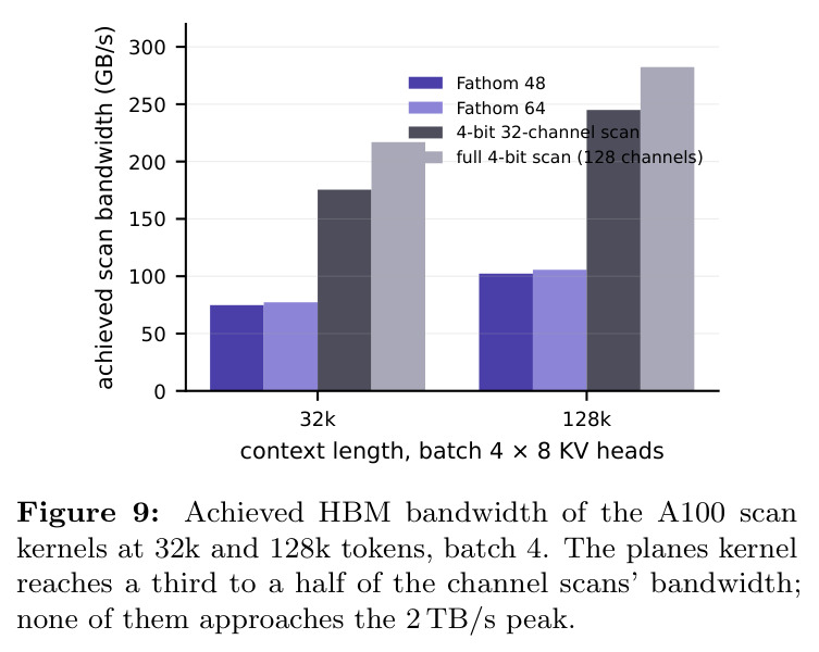
各扫描 kernel 在 HBM 内的实测带宽(32k/128k,batch 4):Fathom 位平面 kernel 只达 75–106 GB/s,nibble 通道扫描 217–245 GB/s,地标索引更低,无一接近 2 TB/s 峰值——因为扫描是算术受限而非带宽受限,位平面每提取 1 bit 的整数操作是 nibble 的四倍。
解释 §7 关键负结果的机制图:为什么索引在 HBM 时方法不更快、为什么融合 kernel 也只能收窄而非消除差距。读懂它才能正确评估方法在其他硬件上的前景。