基于连续深度批处理的循环语言模型深度自适应推理 Depth-adaptive Inference of Looped Language Models via Continuous Depth Batching
首次实现循环语言模型的端到端连续深度批处理推理,把早退的理论加速兑现为99%的实际提升
前置知识
循环语言模型(Looped LM)
把同一个 Transformer 层块(递归核心)反复应用多轮的语言模型。架构分为三段:prelude(进入循环前的处理)、共享递归核心、coda(退出后的输出头),常用 prelude-core-coda 层数配置描述,如 2-4-2 模型在核心跑 $r_t$ 圈时总层数为 $2+4r_t+2$。层共享使其在同等参数量下拥有更大的有效深度,代表工作有 Huginn(隐空间推理)和 Ouro。
本文的全部调度设计与加速分析都围绕这一架构展开,被测的 Ouro(0-24-0 全循环)与 Huginn(2-4-2)正是两类典型代表。
深度自适应解码与早退(early exit)
每个 token 在递归核心里跑的圈数 $r_t$ 由退出准则动态决定:简单 token 少跑几圈省算力,困难 token 多跑几圈保精度。退出准则可以是训练出的退出头(如 Ouro 的 gate),也可以是免训练的收敛判据(如 Huginn 用相邻两步隐状态的归一化 L2 距离低于阈值就退出)。
正是「不同 token 圈数不同」破坏了标准批处理要求 batch 内计算完全一致的前提,直接催生了本文要解决的核心调度难题。
连续批处理(Continuous Batching, CB)
vLLM/Orca 等推理系统的核心调度方式:每个解码步结束后把完成的序列移出、把新序列加入,使 batch 始终保持高占用。它把一次完整前向作为最小调度单元,因此 batch 内所有 token 必须执行完全相同的计算图,只在 token 边界上调度。
CDB 与标准 CB 的对比贯穿全文;理解 CB 为何无法处理变深度前向,才能理解本文的贡献与实验设计。
内存带宽瓶颈与饱和批大小
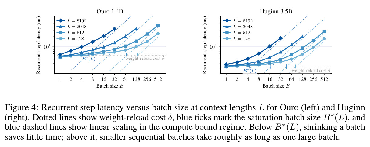
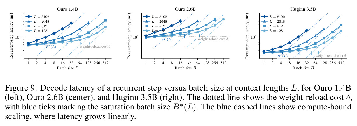
解码时每步都要从显存重新加载全部权重,小 batch 下权重加载时间远超计算时间(memory-bound,计算单元闲置);batch 变大后权重被复用,进入 compute-bound。文中用 $t(B)=\delta+(\gamma+\alpha L)B$ 刻画单步延迟,饱和批大小 $B^*=\delta/(\gamma+\alpha L)$ 是两种机制的转折点,且 $B^*$ 随上下文长度 $L$ 增大而减小。
refill 模式是否有效完全取决于解码处于哪个 regime,这是全文实验设计和「何时该用 refill」结论的关键判据。
KV 缓存与深度索引布局
注意力的键值缓存。深度索引缓存给共享层的每一圈循环分配独立槽位(每 token $r_{max}$ 个槽),早退 token 会留下空槽,导致后续更深层的 token 注意不到它;共享缓存则每层只保留一个槽、每圈覆盖写入,可把递归核心的 KV 内存缩小 $r_{max}$ 倍,但可能损害精度,需要模型兼容。
缺失 KV 状态是 CDB 的三大挑战之一,缓存布局同时影响精度、显存和调度复杂度,是本文重要消融的对象。
研究动机
循环语言模型承诺深度自适应推理:让「简单」token 少跑几圈共享层、「困难」token 多跑几圈,从而在保持精度的情况下省下大量递归计算 FLOPs。但这些 FLOP 节省不会自动转化为实际加速。首先,LLM 自回归解码本身是内存带宽瓶颈:不组 batch 时每步都要把全部权重从显存加载一遍,权重加载时间往往超过计算本身,计算单元大量闲置;只有靠大批处理复用权重才能摊薄加载成本。其次,圈数不同的 token 无法共享同一次均匀前向:已退出的 token 要去跑 coda,留下的 token 还要继续下一圈,而 vLLM/Orca 式连续批处理只在 token 边界调度、把整个前向当作一个调度单元,因此完全无法处理这种变深度前向。Bae 等人虽提出了连续深度批处理(CDB)的概念并用仿真估计了吞吐收益,但其后续消融实验排除了 prefill、调度和 KV 缓存更新的开销——一个朴素的 CDB 实现完全可能因调度开销超过早退收益,反而比标准固定深度批处理更慢。深度自适应推理的实际价值因此悬而未决。
本文的目标是本文要回答两个问题:深度自适应的循环 LM 到底能不能被高效服务?哪些架构性质决定了它的加速上限?为此作者设定了四项具体目标。第一,构建第一个端到端的 CDB 实现,完整覆盖此前被仿真忽略的全部成本:prefill、prelude/coda 等边界阶段的调度、循环间 KV 缓存管理以及异步批准备。第二,推导 FLOP 层面的解码加速上界 $S_{dec}$ 和经过 prefill 校正的端到端上界 $S_{e2e}$,并建立硬件感知的循环步延迟模型,用于预测 refill 何时有效。第三,在两类代表性架构上量化 CDB 能兑现理论加速的百分比:Ouro 1.4B(全循环 0-24-0,$r_{max}=4$)代表边界阶段最小的设计,Huginn 3.5B(2-4-2,$r_{max}=16$,50% 的 Transformer 层在核心外)代表边界层昂贵的设计。第四,从实验中提炼面向推理效率的循环架构设计准则,指导未来的模型-系统协同设计。
与已有工作不同的是,已有循环 LM 研究几乎都从建模和精度角度出发,很少从推理系统视角审视。早退在标准 Transformer 上也被广泛研究过,但其非共享层使得跨深度 refill 困难、缺失的 KV 状态需要重算或近似;循环架构的共享核心天然支持跨深度复用 KV 而无需重算,这正是本文把 CDB 限定在循环 LM 上的理由。与 Bae et al.(2025a)的理论 CDB 以及(2025b)排除 prefill、调度与 KV 更新成本的消融实验不同,本文第一次把所有真实成本纳入端到端实现与评测。独特的切入角度还包括:同时对比「全循环」与「带边界 Transformer 层」两类架构,得出边界阶段成本是核心效率约束这一可操作结论;提出 lookahead gate 解决退出决策的关键路径问题;并用硬件感知延迟模型(饱和批大小 $B^*$)把「refill 何时有效」从经验观察升级为可计算的判据。CDB 本身不改变模型的预测和退出决策,是纯粹的系统能力增强。
核心方法
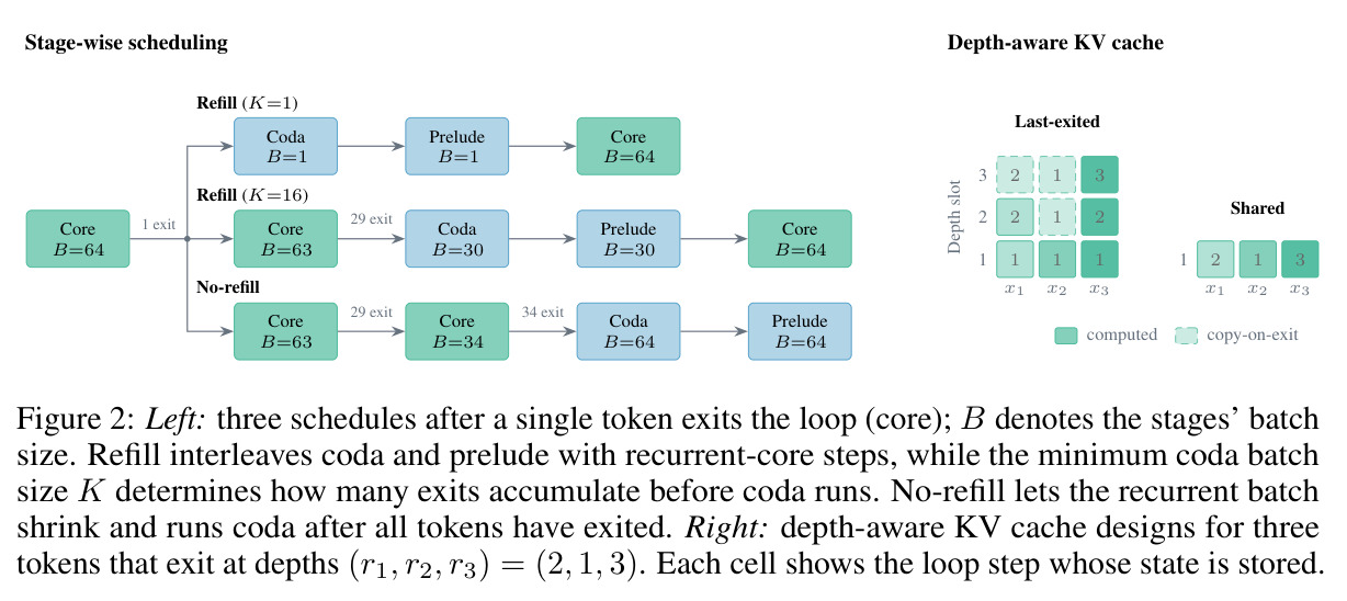
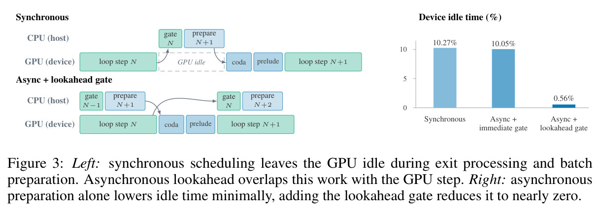
直觉上,CDB 把「一次解码步」这个不可分割的调度单元拆碎,让调度器在圈与圈之间重新组 batch:token 一退出递归核心就把槽位让给新 token,保持 batch 满载。技术路线分四部分。其一,阶段化调度:把每个请求从 prompt 到完成的路径拆成四个队列——等待 prefill 的非活跃请求、等待 prelude 的解码 token、等待下一圈的递归项、等待 coda 的已退出 token,四种 stage 可任意交错执行;提供两种模式,no-refill 固定顺序(prelude→循环至全部退出→coda),batch 只缩不补,refill 则按优先级动态排序(coda>prefill>循环)并用最小 coda 批大小 $K$ 控制攒多少个退出才跑一次 coda。其二,深度感知 KV 缓存:last-exited 缓存在退出时把最终状态拷贝进被跳过的槽位;shared 缓存每层单槽覆盖写,把递归核心 KV 内存缩小 $r_{max}$ 倍。其三,异步调度:CPU 在 GPU 执行当前 stage 时并行准备下一批,配合 lookahead gate 提前一圈做退出决策,把 GPU 空闲时间从 10.27% 压到 0.56%。其四,工程加速:CUDA graphs、静态预分配张量、batch 按 2 的幂 padding、FlashAttention-3 与 paged attention。
核心创新是把调度粒度从「token 边界」细化到「循环步边界」,并让退出与补员在 forward pass 内部即时发生。与标准 CB 的本质区别有二。第一,refill 的替换 token 不是凭空可得的:退出的 token 经 coda 产出后继 token,再经 prelude 直接回到递归队列;新请求完成 prefill 和 prelude 后也汇入同一队列。本文让这两条补给路径与循环步交错执行,从而任何时刻都有候补 token 可填槽——这在架构上要求边界阶段足够便宜,否则补员速度跟不上退出速度。第二,退出决策存在「关键路径」问题:第 $r$ 圈的门控结果决定谁能进第 $r+1$ 圈,若同步等待 GPU 回读结果再组批,GPU 只能空转。本文借鉴推理系统对 EOS「假设不发生、晚一步捕获」的思想提出 lookahead gate:第 $r$ 圈的退出信号决定该 token 是否参加第 $r+2$ 圈而非 $r+1$ 圈,给 CPU 整整一圈的准备时间;与 EOS 方案不同,它把决策提前而非捕获推后,不浪费任何计算。附录 E.2 证明提前一圈决策不损失精度。
方法步骤详情
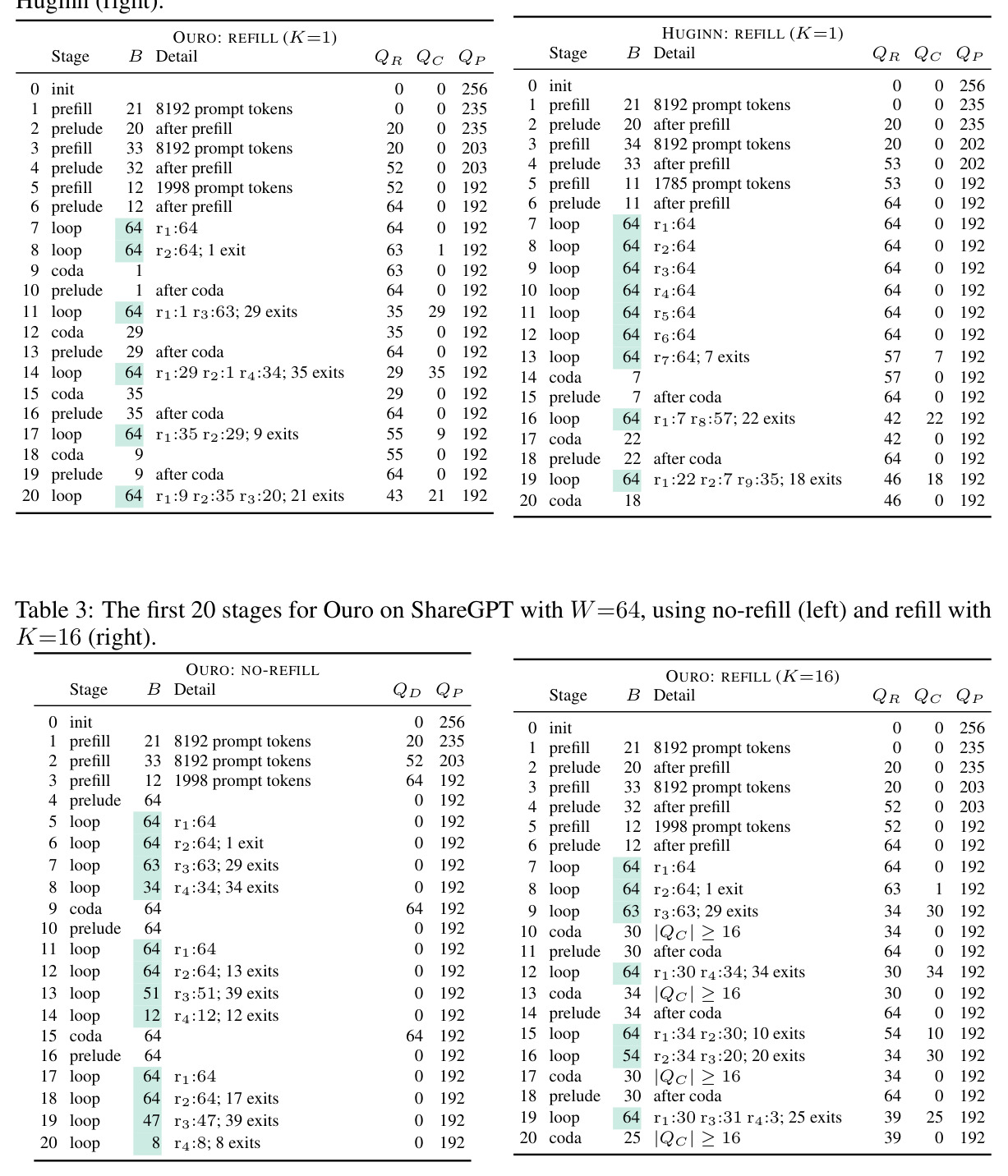
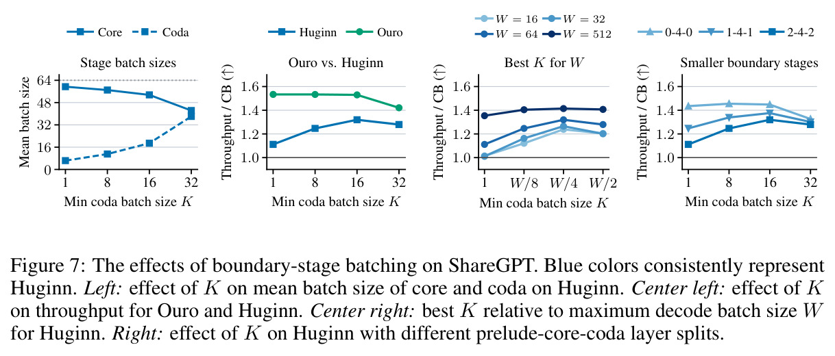
完整流程如下。第一步 prefill:多个 prompt 打包进最多 $M{=}8192$ token 的 prefill 批(chunked prefill,放不下的部分留给下一批),全深度前向产出每个序列的首个生成 token,KV 写入 paged 缓存。第二步 prelude:解码 token 通过 prelude(Ouro 仅嵌入层,Huginn 有 2 层 Transformer),输出进入递归队列 $Q_R$。第三步循环:调度器取出 $Q_R$ 中全部 token 跑一圈共享核心——圈数不同的 token 可混合在同一前向中,因为各圈加载的权重相同;随后门控评估,退出者进入 coda 队列 $Q_C$,其余回到 $Q_R$。no-refill 模式下 $Q_R$ 只缩不补,等全部 token 退出后一次性跑 coda;refill 模式按优先级调度:$Q_C$ 攒够 $K$ 个就跑 coda(Ouro 取 $K{=}1$,Huginn 取 $K{=}W/4$),coda 产出的后继 token 立即接 prelude 回填 $Q_R$;否则若满足准入条件就跑 prefill;否则跑循环。第四步 KV 处理:深度索引缓存下用 last-exited 策略在退出时把最终 KV 拷入空槽;shared 缓存每层单槽覆盖写,深层 token 自动看到各早退 token 的最新状态。第五步异步执行:为 prelude、核心、coda 分别预录制 CUDA graph,张量静态预分配、batch 按二的幂 padding;CPU 在 GPU 执行当前 stage 时异步完成回读、选批与数据搬运,lookahead gate 提前一圈给出退出信号。附录 Table 2/3 的 20 步调度 trace 给出了每步输入输出与批大小的完整示例。
技术新颖性
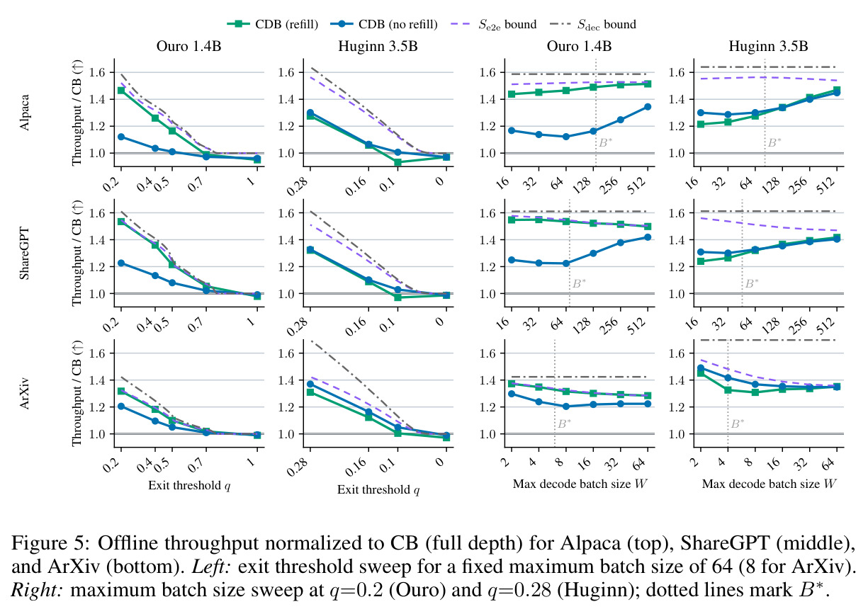
技术新颖性体现在四点。第一,首个端到端 CDB 实现:此前只有仿真估计(Bae 2025a)和排除 prefill、调度、KV 更新成本的消融(Bae 2025b),本文补齐全部真实成本,证明全循环架构可兑现理论加速的 96–99%。第二,系统的理论刻画:解码 FLOP 上界 $S_{dec}=\frac{F_0+r_{max}F_r}{F_0+\bar{d}F_r}$、prefill 校正的端到端上界 $S_{e2e}=(\alpha+(1-\alpha)/S_{dec})^{-1}$,以及循环步延迟模型 $t(N_c,N_b)=\delta+\gamma N_b+\alpha N_c$ 与饱和批大小 $B^*=\delta/(\gamma+\alpha L)$,把「refill 何时有效」变成可计算判据——memory-bound 区间(batch 低于 $B^*$)refill 收益最大。第三,lookahead gate 是首个在批处理环境下解决退出决策关键路径的机制,比 EOS 式晚捕获方案不浪费计算,且经训练验证精度无损。第四,架构层面的对照结论:全循环(Ouro 0-24-0)最适合深度自适应推理,昂贵的边界 Transformer 层(Huginn 2-4-2)会拖慢并复杂化调度,为推理感知的循环 LM 设计提供了直接依据。
实验结果
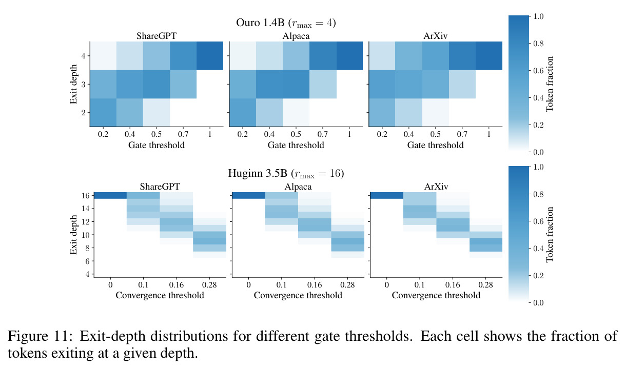
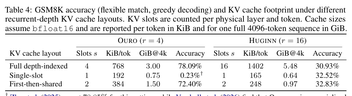
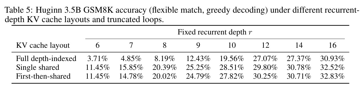
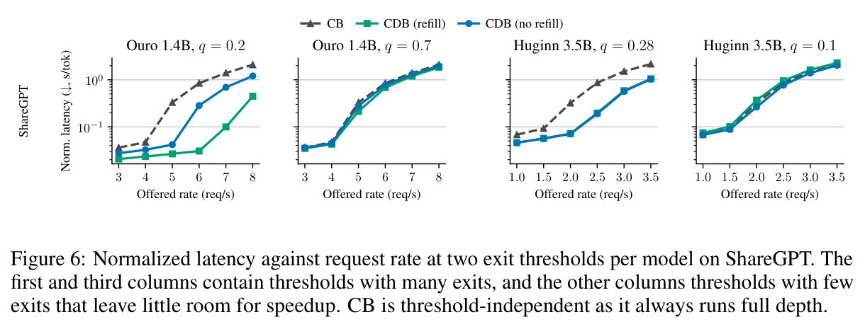
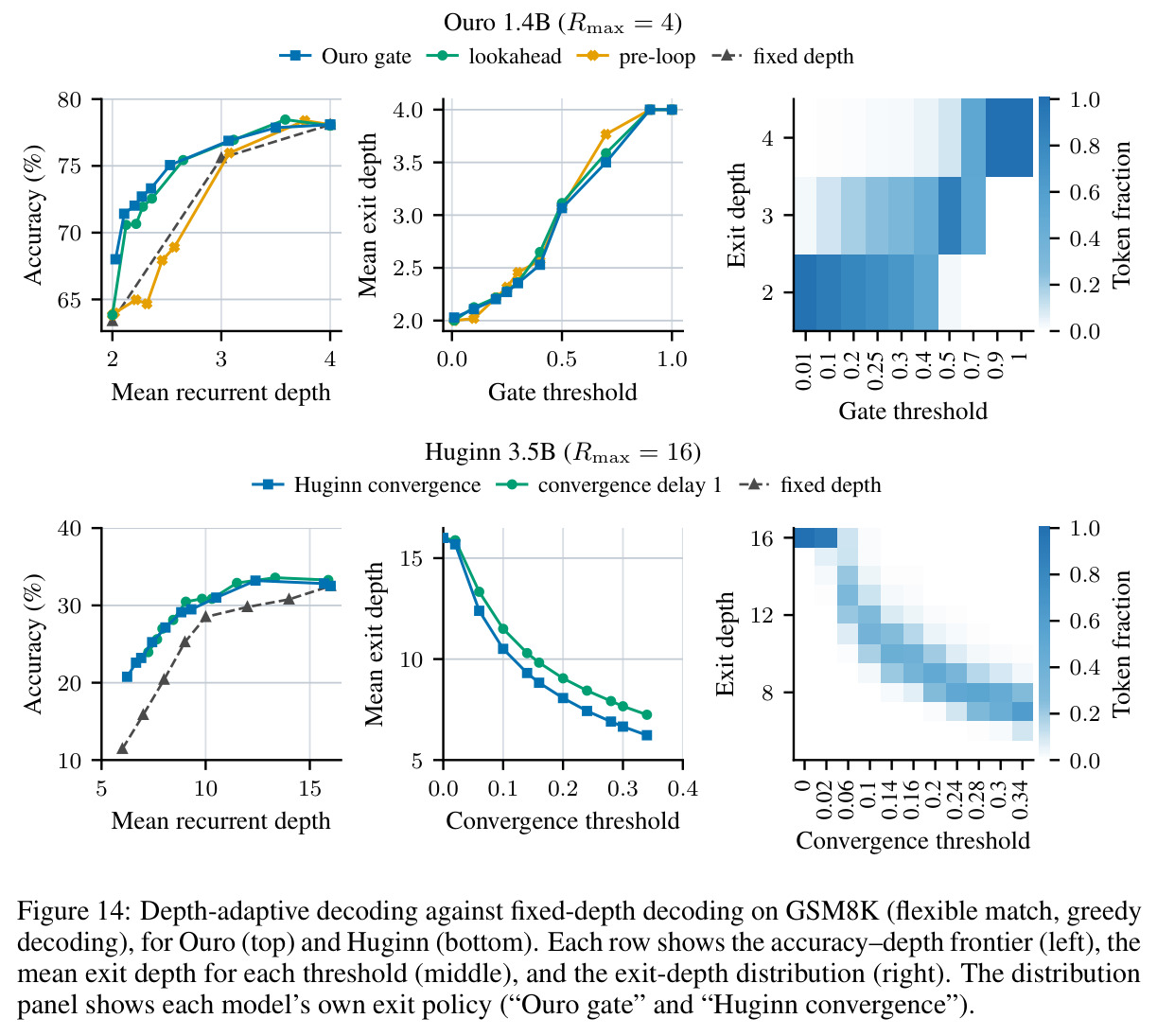
实验在单张 80GB H100 上进行,对比 CDB(refill/no-refill)与标准 CB。离线吞吐方面(最大解码批 $W{=}64$,ArXiv 用 8):在选定阈值下,Ouro 上 refill 达到 CB 的 1.32–1.53 倍吞吐,兑现 prefill 校正上界 $S_{e2e}$ 的 96–99%;Huginn 上 no-refill 更优,达 1.30–1.37 倍,兑现 83–96%。全深度(无早退)时 CDB 仍保留 CB 吞吐的 95–99%,说明分阶段前向与调度交互的开销很小。refill 的优势在 batch 接近或低于饱和批大小 $B^*$(memory-bound 区)时最大,batch 增大进入 compute-bound 后收窄,与延迟模型预测一致。prefill 占 GPU 时间的 3.7–36%(ArXiv 长上下文最高),因此 $S_{e2e}$ 在 ArXiv 上显著低于仅看解码的 $S_{dec}$。延迟测量:Ouro 1.4B 权重重载成本 $\delta\approx 5.4$ ms(1.2B 参数分布在 24 个窄层),Huginn $\delta\approx 2.3$ ms(1.6B 参数分布在 4 个宽层);Ouro 的 $B^*$ 从 $L{=}128$ 时约 140 降到 $L{=}8192$ 时的个位数,Huginn 从约 80 起类似下降。在线服务(Poisson 到达、10 分钟窗口、报告归一化延迟):CDB 能在更高请求率下才出现延迟拐点,把离线吞吐增益转化为服务容量;Ouro 的 refill 容量增益最大、no-refill 约为其一半,Huginn 两种模式容量相同。消融:最小 coda 批大小 Ouro 取 $K{=}1$ 最优、Huginn 取 $K{=}W/4$ 最优;把 Huginn 改为全循环 0-4-0 后 $K{=}1$ 变为接近最优,且与上界的差距缩小,证实边界层成本是核心约束。异步调度把 GPU 空闲从 10.27%(同步)降到 10.05%(仅异步)再到 0.56%(异步+lookahead gate)。精度侧(GSM8K):KV 共享对 Huginn 无损甚至有益(深度索引 30.93% → 单槽 32.52%),对 Ouro 单槽共享则崩溃(78.09% → 0.23%),first-then-shared 损失约 5.7 点;深度自适应解码 Pareto 支配固定深度解码,Ouro 可降到平均深度约 2.5、Huginn 约 8;lookahead gate 与教师门精度和阈值曲线基本一致。
查看结构化数据
| 任务 | 指标 | 本文 | 基线 | 提升 |
|---|---|---|---|---|
| 离线吞吐 · Ouro 1.4B(Alpaca/ShareGPT/ArXiv,W=64) | 相对标准 CB(全深度)的吞吐加速比 | CDB (refill) 1.32–1.53× | 标准 token 级 CB 1.0× | 兑现 prefill 校正上界 $S_{e2e}$ 的 96–99%,接近理论最大加速 |
| 离线吞吐 · Huginn 3.5B(同上工作负载) | 相对标准 CB 的吞吐加速比 | CDB (no-refill) 1.30–1.37× | 标准 CB 1.0× | 兑现 $S_{e2e}$ 的 83–96%;昂贵边界层使 refill 不如 no-refill |
| 调度开销(全深度、无早退) | 相对 CB 的吞吐保留率 | 95–99% | CB 100% | 分阶段调度额外开销仅 1–5% |
| GPU 空闲时间(调度异步化消融) | 设备空闲时间占比 | 0.56%(异步 + lookahead gate) | 同步调度 10.27%(仅异步为 10.05%) | 空闲时间降至约 1/18 |
| 递归核心 KV 缓存内存(单槽共享布局) | 每 token 缓存占用 / GSM8K 精度 | Ouro 192 KiB/tok(精度 0.23%,崩溃);Huginn 165 KiB/tok(精度 32.52%,反升) | 深度索引布局:Ouro 768 KiB/tok(78.09%)、Huginn 1402 KiB/tok(30.93%) | 内存分别缩小 4× 与 8.5×;Huginn +1.59 点,Ouro 需 first-then-shared(72.40%)兜底 |
| 在线服务容量(ShareGPT,Poisson 到达,10 分钟窗口) | 归一化延迟拐点对应的可维持请求率 | CDB 在显著更高的请求率下延迟才上扬;Ouro 上 refill 增益最大 | 标准 CB | Ouro 的 no-refill 容量增益约为 refill 的一半;Huginn 两种模式持平;退出少的阈值下优势消失 |
局限与改进
作者承认的局限:只评测了两个循环架构、单张 H100 GPU;未来的循环模型可能引入混合专家等改变递归与边界阶段成本的组件;实验未包含生产级服务特性(多卡执行、抢占、前缀缓存、投机解码),这些技术可能改变 prefill 与解码的平衡或与深度自适应调度产生新的交互,CDB 的相对收益在完整服务系统中可能不同。我自己的观察:其一,实验中退出决策是离线录制后回放的,不是在线闭环,未计入门控网络自身的计算与调度开销,也未反映真实服务中的反馈效应;其二,KV 共享结论两极分化——Ouro 单槽共享崩溃到 0.23%,与原论文声称的近无损 KV 共享相矛盾,说明 shared cache 并非普适,落地必须逐模型验证;其三,lookahead gate 需要额外的蒸馏训练且强加最小退出深度 $r_{min}{=}2$,对可能在 1 圈后就能产出有用结果的浅层模型不友好;其四,$K$、退出阈值等超参需按模型手工调优(Ouro 用 $K{=}1$、Huginn 用 $K{=}W/4$),缺少自适应选择机制;其五,基线是作者自研的 CB 引擎而非完整的 vLLM/SGLang 生产配置(如 piggybacking 混批被有意关闭),绝对吞吐数字与生产系统的横向可比性有限。
独立分析的弱点
第一,lookahead gate 的 $r_{min}{=}2$ 约束与训练成本:需要用 Nemotron 数据集做门控蒸馏,且排除了 1 圈退出的可能,对浅循环模型会直接压缩可加速空间。改进方向:按作者建议先在进入核心前预测「第一次退出」、之后各圈用 lookahead 决策,实现 $r_{min}{=}1$ 而无需预知完整退出深度。第二,KV 共享精度不可移植:Ouro 单槽共享 GSM8K 崩到 0.23%,last-exited 拷贝又引入拷贝开销并保留 $r_{max}$ 倍内存。改进:把 KV 共享纳入训练目标(如 Vendrell et al. 的微调方案),或探索 first-then-shared 等混合布局(Ouro 损失已收窄到约 5.7 点)。第三,refill 依赖候补 token 供给:边界层昂贵时 coda/prelude 无法频繁运行、槽位补不上,Huginn 上 refill 反而不如 no-refill 就是例证。改进:降低边界阶段成本(缓存 prelude 输出、压缩 coda),或按 $B^*$ 与队列水位自适应选择 $K$ 与 refill/no-refill 模式。第四,评测设定的理想化:退出序列离线录制、抢占关闭、无前缀缓存/投机解码/MoE;真实服务的排队与内存压力会改变 $B^*$ 与最优模式。改进:接入完整生产引擎做闭环评测。第五,只覆盖 1.4B/3.5B 的 dense 模型:更大模型权重加载成本 $\delta$ 更大、$B^*$ 更小,refill 理论上更有利,但 KV 与激活显存压力也更大,结论外推需要验证。
未来方向
作者提出的方向:一是训练能在目标精度下提供更多早退的模型——CDB 已证明系统侧可兑现约 99% 的可用加速,剩余收益主要来自更频繁且可靠的退出行为;二是循环架构与推理系统协同设计:保持循环外阶段尽量小(在精度收益与推理效率间权衡)、谨慎选择循环数(圈数多则退出粒度细但每圈节省占比小,且 iso-depth 缩放律显示高圈数损精度)、设计可靠支持 KV 共享的模型布局;三是退出门设计:预测核心前的首次退出以解除 $r_{min}{=}2$ 约束,而完整的退出深度预测已知不可靠;四是在更广的服务系统(多卡、抢占、前缀缓存、投机解码、MoE)中检验 CDB 收益的变化。基于本文成果可延伸的:把 $B^*$ 判据做成在线控制器,自动在 refill/no-refill 间切换并动态调 $K$;将 CDB 与 prefill/decode 混批(piggybacking)结合;把深度自适应调度与投机解码的草稿-验证机制结合;研究 CDB 与 Mixture-of-Depths 式固定组退出的混合调度;以及在 RL 训练和批量评测这类离线高吞吐场景(本文明确的应用画像)中做工程化部署。
复现评估
复现基础较好。模型侧:Ouro 1.4B 与 Huginn 3.5B 均为公开权重的开源模型;数据侧:Alpaca、ShareGPT、ArXiv-Summarization 以及用于门控蒸馏的 Nemotron-Post-Training-Dataset-v2 全部公开;工程细节方面,附录 A 给出近乎完整的实现说明——Table 1 列出全部参数($M{=}8192$、$W$ 扫描集、上下文 16384、KV 块大小 16、bfloat16、Paged FlashAttention-3、CUDA graphs 等),Algorithms 1/2 给出两种模式的伪代码,Tables 2/3 给出 20 步调度 trace,附录 B 给出延迟拟合方法。硬件门槛:单张 80GB H100,消费级显卡难以复现绝对延迟数字,但相对结论(refill 在 memory-bound 区更有利、边界层成本影响)应可迁移。主要难点:论文未明确承诺开源代码,引擎基于 HF Transformers 加 vLLM/SGLang 组件自研,完整复现需要自行实现 CDB 调度器、深度感知 KV 缓存、异步执行与分段 CUDA graph 捕获,系统工作量不小;门控蒸馏与 GSM8K 评测部分复现相对直接。总体属于「中高难度、信息充足」的系统类复现。
论文图表
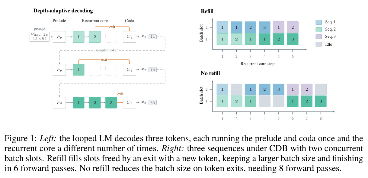
左图展示循环 LM 的三段式解码:prelude 与 coda 各跑一次,递归核心按 token 难度跑不同圈数(如「What」「is」各 1 圈即可退出,而「12×5?」需要 3 圈才得出 60)。右图对比 CDB 的 refill 与 no-refill:三个序列、两个并发槽位下,refill 在 token 退出后立即补入新 token,保持大批处理,6 次前向完成;no-refill 只删不补,batch 逐渐缩小,需要 8 次前向。
这是全文问题与方法的总示意图:一眼看懂深度自适应解码是什么、为什么标准批处理失效、以及 refill 为何能省下 2 次前向。理解这张图就理解了论文的出发点。
列出主实验的全部推理配置:最大序列数 W=64(批扫描时 2–512)、最大批 token 数 M=8192、最小空槽 S=max(1,⌊W/8⌋)、上下文 16384、KV 缓存 20480 块(327680 token 位)、块大小 16、shared 缓存布局、最小 coda 批 K(Ouro 为 1、Huginn 为 ⌊W/4⌋)、bfloat16、Paged FlashAttention-3、prefill 与 decode 均启用 CUDA graphs,抢占关闭。
系统论文的复现命脉:所有延迟、吞吐数字都依赖这些参数,附录 A 逐项解释了每个参数的作用机理。
逐步列出 refill 模式前 20 个调度 stage 的批大小、队列水位与细节(如 stage 14 把处于第 1、2、4 圈的 token 混入同一次前向)。可以看到 Ouro 的 coda/prelude 几乎每个退出后都立即执行(K=1),核心批全程保持 64;Huginn 因边界层贵,退出攒到一定量才跑 coda。
把抽象的调度算法变成可逐步核对的 concrete trace,是理解「不同圈数 token 如何混合前向」和 refill 实际运作方式的最佳材料。