极简视觉惯性里程计:仅用4个带光学Gabor掩模的光电二极管实现平面里程计 Minimalist Visual Inertial Odometry
4像素+IMU的差速驱动里程计,仿真训练零样本迁移到真实场景
前置知识
视觉惯性里程计 (VIO)
融合相机图像与惯性测量单元 (IMU) 数据的定位技术,通过关联连续帧的视觉特征并积分IMU加速度/角速度,估计机器人6自由度位姿。传统VIO需要处理高分辨率图像流,计算与功耗开销巨大。
本文直接对标VIO,指出其高像素开销在资源受限机器人上的瓶颈,是理解论文动机和对比基线的必备基础。
Gabor滤波器
由高斯包络调制的正弦波函数,在频域具有最优的时频局部化特性,能精确提取特定空间频率 $\xi_0$ 及其邻域成分。本文把Gabor作为光学掩模的形状先验,使光子在模拟域完成空间滤波。
Gabor是本文硬件设计的核心数学工具,作者论证了它在运动感知中的理论最优性,是理解频域分析 $f_0=\xi_0 v$ 公式的前提。
时序卷积网络 (TCN)
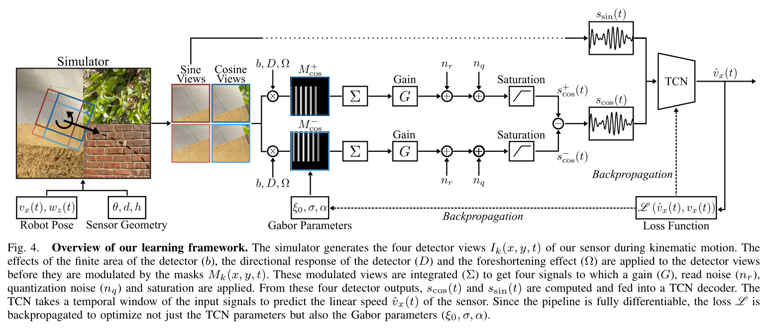
使用因果膨胀卷积处理一维时序信号的深度网络,通过多层膨胀卷积获得指数级感受野。本文中的TCN仅18.4万参数,从1秒窗口 (2×1000采样) 的两个信号 $s_{\cos}(t)$、$s_{\sin}(t)$ 中回归线速度 $\hat{v}_x(t)$。
TCN是与Gabor掩模联合训练的软件解码器,理解其输入输出形式对把握端到端学习框架至关重要。
可微仿真器
仿真管线中所有算子 (图像变换、卷积、噪声注入、积分) 都支持梯度反向传播,使损失信号可一路回传到掩模参数 $(\xi_0, \sigma, \alpha)$,实现『硬件+软件』协同设计。
这是本文方法论的关键支撑,使得掩模几何参数能被梯度优化而非手工调参。
差速驱动运动学
两独立驱动轮的小车模型,位姿变化由线速度 $v_x$ 与偏航角速度 $\omega_z$ 完全确定。本文将4像素传感器测得的 $v_x$ 与IMU陀螺仪测得的 $\omega_z$ 融合,得到完整平面轨迹 $(x, y, \theta)$。
理解本文为何只需估计 $v_x$ 而非完整6DOF位姿,是把握系统简化逻辑的前提。
研究动机
传统视觉惯性里程计 (VIO) 在资源受限移动机器人上存在显著的功耗与算力瓶颈:相机图像传感与处理的能耗大致随像素数线性增长,单个高分辨率图像传感器通常消耗数百毫瓦,加上视频流特征提取与匹配的开销,使长时间自主运行的小型平台难以承受。轮式编码器虽能给出短期基线,但在户外/打滑场景下漂移严重;纯IMU方案通过对加速度二次积分估计位置,漂移更快。本文作者在多个数据集 (TartanGround, 80公里、12小时轨迹) 和实地 (920米、87分钟室内外混合) 场景中均观察到这类权衡,并明确指出低功耗是差速驱动机器人的核心痛点。
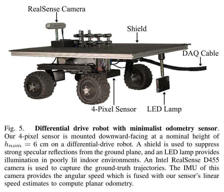
本文的目标是本文追求『用最少感知资源实现稳健平面里程计』的设计目标。具体而言,希望摆脱高分辨率成像,把外感受传感器压缩到 4 个朝下的光电二极管 (4个像素),每个二极管前放置一个光学掩模用于在模拟域做空间滤波;将得到的4路时域信号送入一个轻量时序卷积网络 (TCN,约18.4万参数),实时回归线速度 $\hat{v}_x$;再与IMU陀螺仪的偏航角速度 $\omega_z$ 融合,得到完整 $(x, y, \theta)$ 平面轨迹。系统端到端功耗目标为mW量级,相比传统相机降两个数量级。
与已有工作不同的是,已有『极简视觉』工作 [Pooj et al. 2018, Klotz & Nayar ECCV 2024] 已证明可以用少量掩模像素做目标识别与自由形式像素回归任务,但前者面向识别而非运动估计,后者让掩模完全自由学习。在本文要解决的『速度估计』问题上,自由掩模缺乏频域局部化先验会收敛到模糊图案 (仿真验证RMSE=0.147 m/s,远差于Gabor先验),因此本文的独特切入点是:把运动感知的『时空频率分析』理论与Gabor滤波器的『最优时频局部化』性质结合,把掩模约束为参数化Gabor函数 $(\xi_0,\sigma,\alpha)$ 并通过可微仿真器与TCN联合优化——既保留物理可解释性,又获得数据驱动的鲁棒性。
核心方法
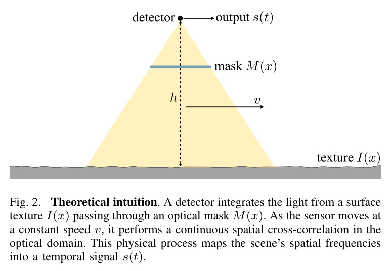
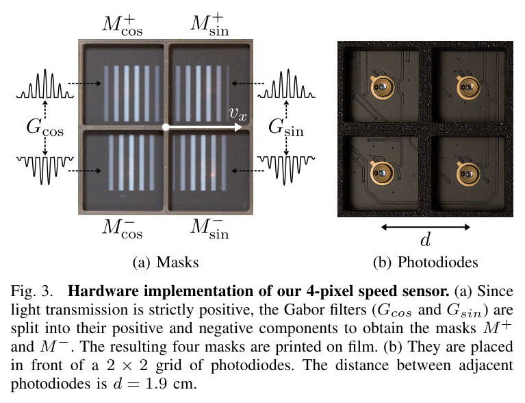
整体思路遵循『光学域模拟计算 + 数字域轻量解码』的极简范式。直觉层面,作者把『运动』重新理解为『时空频率的平移』:当传感器以速度 $v$ 掠过地面纹理时,每个掩模像素的光电流相当于对纹理做空间互相关 $S_x(x)=(I\star M)(x)$,等效于在模拟域实现『空间频率 $\xi$ 到时间频率 $f=\xi v$』的映射;只要掩模是中心频率为 $\xi_0$ 的窄带滤波器,输出信号的基频 $f_0=\xi_0 v$ 就直接编码速度。技术路线分为三步:(1) 用 cos/sin Gabor 对解决方向模糊,并把 Gabor 拆成4个非负掩模 $M_{\cos}^+,M_{\cos}^-,M_{\sin}^+,M_{\sin}^-$ 印在透明胶片上;(2) 搭建可微物理仿真器,用 Matador 纹理集 + TartanGround 轨迹生成4路带噪声的传感器信号;(3) 训练一个184K参数的TCN解码器,并通过反向传播同时优化掩模的 $(\xi_0,\sigma,\alpha)$ 与TCN权重,得到可直接打印的物理掩模 + 即用即推理的解码网络。
核心创新有三点,与已有方法形成本质区别:第一,『频域里看运动』的理论等价——证明带Gabor掩模的光电二极管本质上是窄带时空频率滤波器,把传统VIO中『特征点匹配→光流估计→运动解算』的多级数字流水线压缩为『光学互相关→频率检测』两级物理过程;第二,方向歧义的『正交双相化解法』——单个Gabor掩模只能给出 $|v|$ 而丢失符号,通过部署 cos/sin 两个相位差90°的掩模对,使前向/反向运动在两路信号相对相位 $\pm 90°$ 上可区分,这是无需高帧率或事件相机就能解决方向二义性的新颖解;第三,『光学硬件 + 神经网络』端到端联合设计——区别于自由像素方法让掩模完全自由学习(仿真RMSE 0.147 m/s),本文把Gabor频域局部化作为强先验,仿真RMSE降到0.054 m/s,相对降幅29%,同时掩模仍具物理可解释性、可印刷。
方法步骤详情
方法分四步。步骤1:硬件——把 Gabor(参数 $\xi_0,\sigma,\alpha$)拆为 4 个 16×16 mm² 非负掩模($M^+=\max(G,0)$、$M^-=\max(-G,0)$),胶片打印于 Hamamatsu 二极管 2×2 阵列前(间距 1.9 cm、视场 70°、$h_{nom}=6$ cm)。步骤2:可微仿真器——Matador (7200 张、57 类) + TartanGround (80 km) 生成 4 路 128×128 灰度图,依次施模糊、方向响应、缩短、掩模调制、积分、增益与噪声,组合得 $s_{\cos}$、$s_{\sin}$。步骤3:训练数据——1000 Hz 上采样轨迹 + $\Delta h\in\pm 25\% h_{nom}$ 模拟振动,1秒窗口产 2×1000 输入。步骤4:优化——184K 参数 TCN 用膨胀卷积+注意力池化+残差头输出 $\hat{v}_x$ 与 $\log\hat{\sigma}^2$,高斯负对数似然损失;仿真器可微使梯度回传 $(\xi_0,\sigma,\alpha)$,得可印刷掩模+即用网络。
技术新颖性
技术新颖性体现在四个层面:(1) 把『时空频率分析』理论与『光学模拟计算』硬件结合,把Gabor掩模从数字图像处理工具变为物理感知器件,并给出完整的频域等价性证明 (Eq. 1–2 的 $f=\xi v$ 推导);(2) 解决方向模糊的『正交双相化』解法不依赖事件相机或多像素阵列,仅用 cos/sin Gabor 对就实现 $\pm 90°$ 相对相位编码;(3) 端到端可微仿真器支持『掩模几何参数 + 网络权重』同时优化,是协同设计光学硬件与神经网络的代表性范例;(4) 在差速驱动机器人上完成 920 m、87 min 真实室内外测试,仿真训练零样本迁移,ATE 0.28 m / 漂移 0.60%,相对轮编码器+IMU基线提升约 60% 的 ATE 性能。
实验结果
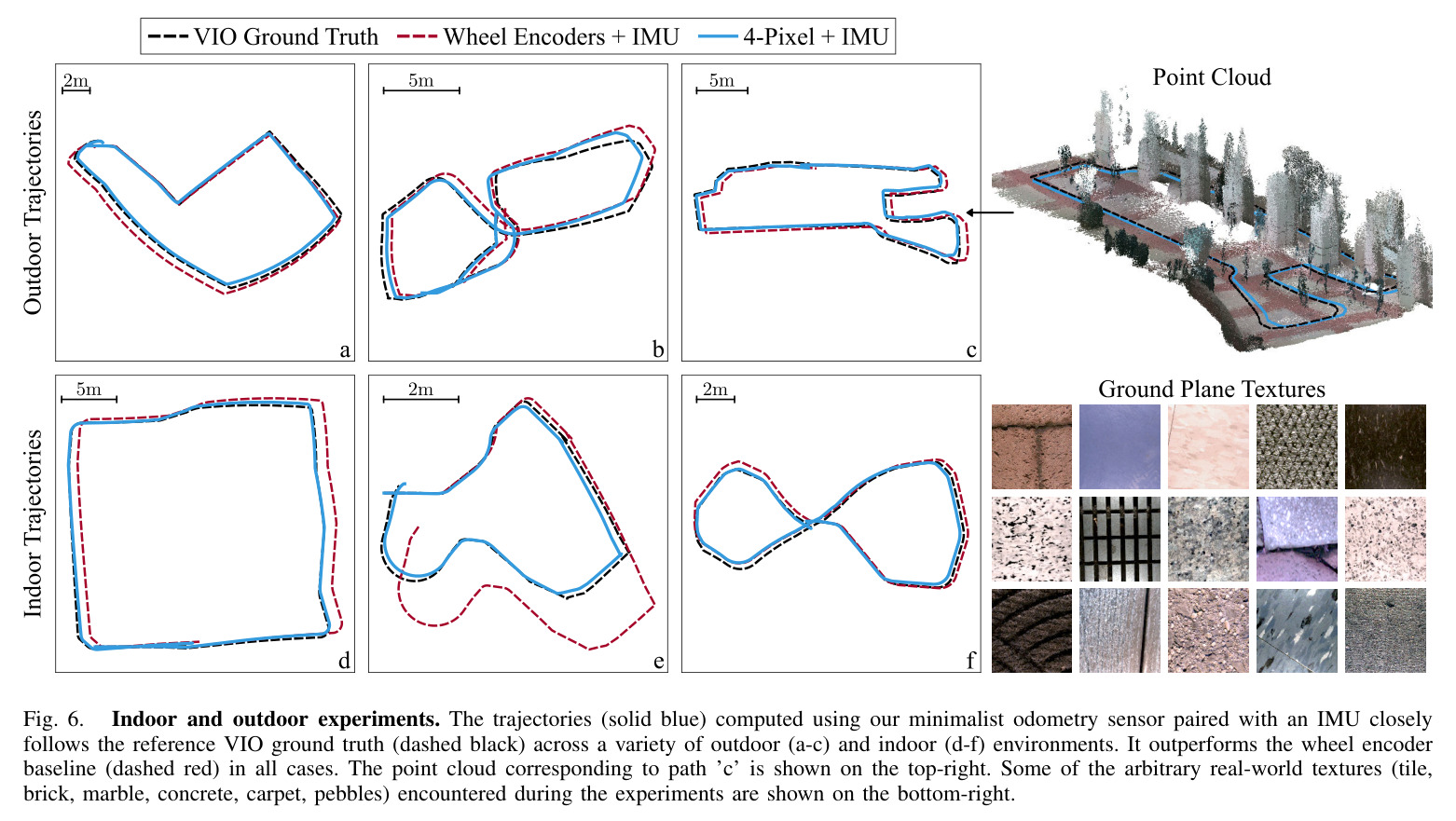
仿真 (Table I):Freeform 像素缺频域先验最差 (RMSE 0.147 / MAE 0.101 m/s),Fixed Gabor ($\xi_0=6,\sigma=1,\alpha=1$) 0.076 / 0.052,Learned Gabor 联合优化后 0.054 / 0.034,相对 Fixed 降低 29% / 35%。Table II:固定高度训练在 $\pm 50\%$ 偏移测试时 RMSE 跳到 1.542 m/s;$\pm 25\%$ 高度扰动训练后保持 ≤ 0.056。真实 (Table III, 11 室内+5 室外共 920 m / 87 min):室内 4-Pixel+IMU (1 kHz) ATE 0.28±0.11 m / 漂移 0.60±0.22%,优于 Encoders+IMU (0.75±0.47 m / 1.62±1.66%);室外 ATE 0.42±0.08 m / 0.62±0.25%,优于 0.74±0.19 m / 1.37±1.20%。降频 100/30 Hz 几乎不变。功耗 4 像素仅 2.5 mW,比相机降约100x。
查看结构化数据
| 任务 | 指标 | 本文 | 基线 | 提升 |
|---|---|---|---|---|
| 差速驱动室内里程计 (11条轨迹, 618 m, 61 min) | ATE (m) ± std / 端点漂移 (%) ± std | 4-Pixel + IMU (1 kHz): 0.28 ± 0.11 m / 0.60 ± 0.22% | Encoders + IMU: 0.75 ± 0.47 m / 1.62 ± 1.66% | ATE 降低约 63%、漂移降低约 63% |
| 差速驱动室外里程计 (5条轨迹, 306 m, 26 min) | ATE (m) ± std / 端点漂移 (%) ± std | 4-Pixel + IMU (1 kHz): 0.42 ± 0.08 m / 0.62 ± 0.25% | Encoders + IMU: 0.74 ± 0.19 m / 1.37 ± 1.20% | ATE 降低约 43%、漂移降低约 55% |
| 仿真速度估计 (固定纹理, Matador + TartanGround) | RMSE (m/s) / MAE (m/s) | Learned Gabor (联合优化): 0.054 / 0.034 | Fixed Gabor ($\xi_0=6,\sigma=1,\alpha=1$): 0.076 / 0.052;Freeform Pixels: 0.147 / 0.101 | 相对 Fixed Gabor RMSE 降低 29%、MAE 降低 35%;相对 Freeform 像素 RMSE 降低 63% |
| 高度鲁棒性 (仿真, 测试 ±10% 高度偏移) | Speed RMSE (m/s) | 训练时使用 ±25% 高度扰动: 0.054 | 训练时使用固定 $h_{nom}$: 0.266 | RMSE 降低约 80%,说明联合训练把高度-相位-频率关系学进了参数 |
| 功耗对比 | 传感器持续功耗 (mW) | 4-Pixel 自研传感器: 2.5 mW | 传统高分辨率图像传感器: 数百 mW | 功耗下降约两个数量级 (~100x) |
局限与改进
作者明确点出的局限与可观察到的隐含限制如下:(1) 仅估计 $v_x$ 单方向速度,没有横向/纵向自由度,机器人必须保持差速驱动且只能在平面运动 (作者已说明未来可扩展到更高自由度平台);(2) 方向歧义由 cos/sin 正交对解决,但要求 $s_{\cos}$ 与 $s_{\sin}$ 通道间的相对相位严格保持 90°,振动、离地高度突变、横向打滑都会破坏此假设,在 §III-C 中作者承认需靠训练中的高度扰动隐式学习缓解;(3) 训练完全依赖仿真,仿真器对真实光照、镜面反射、阴影做了简化 (论文中提到加了挡板和补光LED),室外强光场景仍可能失败;(4) 仿真实验中 $\pm 50\%$ 高度偏移下 RMSE 跳升到 1.5 m/s 量级,表明模型对极端悬架姿态鲁棒性不足;(5) 940 nm 附近光电二极管 + LED 主动补光的方案对极低光或纯被动光环境有限制;(6) 当前 TCN 在 1 kHz 下仍有实时性需求,需配合外部 DAQ (41.6 kHz 采样),端到端嵌入式实现尚未完成 (作者列为未来工作)。
独立分析的弱点
独立分析可观察到以下弱点:(1) 掩模光学频率 $\xi_0$ 全局共享,难以适配『高速小纹理』与『低速大纹理』两种工况,可设计双频段掩模 (4 像素拆为两组用不同 $\xi_0$) 扩展速度量程;(2) 横向位移完全由陀螺仪积分贡献,遇磁场/温漂时融合易出现扭角偏差,可用差速驱动运动学约束 $\dot{\theta}\cdot b=v_R-v_L$ 做闭环校验;(3) 仿真器对镜面反射、雨雪、透明玻璃等『非漫反射』场景建模薄弱,作者靠挡板+补光绕开,根本解决需把 BRDF 多样性纳入纹理集;(4) 训练在 80 km 轨迹+7200 张纹理上仅做监督学习,可加域随机化 (雨雪纹理、振动频谱) 增强极端工况鲁棒性;(5) 1 秒窗口 TCN 在急转弯时相位剧烈变化,单点回归误差会被积分放大,建议同时显式回归 $\dot{v}_x$ 做 IMU 预测-修正;(6) RTAB-Map 评测并非真实地面真值,建议补充动作捕捉或 LiDAR-惯性 SLAM 作为 gold standard。
未来方向
作者明确提出的方向:(1) 设计嵌入式硬件承载优化版 TCN,实现真正 on-board、mW 量级的实时解算;(2) 把掩模设计扩展到 2D/3D 自由度的运动估计,使方法适配无人机等非完整约束平台。可延伸的研究:(3) 用类似『光-频-运动』框架解决地形分类、避障等其他机器人感知任务 (作者已点到);(4) 探索多尺度 Gabor 掩模组,把 $\xi_0$ 做成可学习的多频率集合以扩展量程;(5) 把端到端可微仿真范式推广到事件相机、神经形态传感器等其他极简感知器件;(6) 联合优化掩模几何 + 主动照明频谱 (例如特定波长 LED),提升低 SNR 工况的稳健性;(7) 用自监督或 sim-to-real 域适应进一步缩小仿真到真实的差距,例如引入光线追真渲染 (NeRF/Replica) 替代 Matador 静态纹理。
复现评估
复现友好度整体较高:(1) 仿真器代码已开源 (github.com/pastifra/four-pixel-vio),含 Matador 纹理集引用与 TartanGround 数据生成脚本;(2) 仿真 Table I–II 的超参 ($h_{nom}$=20 cm, $d$=1.9 cm, FOV=70°, 100 epoch, Adam lr=$10^{-4}$, batch=32) 都在论文中给出,可直接基于开源仿真器复现三组对比;(3) 真实硬件依赖 Hamamatsu S9119-01 光电二极管、透明胶片打印、LeoRover 差速底盘、Intel RealSense D455 与外部 DAQ,材料清单明确,但掩模印刷精度与 11.4 mm 探测器-掩模对齐需要定制夹具,复现门槛中等;(4) 训练算力未明确披露,184K 参数 TCN 与仿真管线在单卡 RTX 3080 级 GPU 上数小时可完成 100 epoch;(5) 与 RTAB-Map 的真实对比需自行搭建 920 m 室内外采集系统。总体而言仿真可一键复现,硬件与真实评测需要中等工程投入。
论文图表
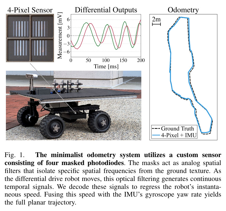
Teaser 图,左侧为论文题目与作者署名 (Francesco Pasti, Jeremy Klotz, Nicola Bellotto, Shree K. Nayar),右侧给出系统示意:一个差速驱动小车上挂着由 4 个朝下光电二极管组成的极简传感器,每个二极管前贴有一片印刷着不同 Gabor 掩模的胶片;传感器底面被屏蔽以避免强镜面反射,并配有 LED 灯用于暗光补光。
以最直观的形式呈现『4像素 + IMU = 平面里程计』的极简范式,是论文 idea 的缩影;放在 motivation 部分能让读者第一眼把握全文要解决的问题与方案。
三行三列仿真结果:Freeform Pixels RMSE 0.147 m/s / MAE 0.101 m/s;Fixed Gabor ($\xi_0=6,\sigma=1,\alpha=1$) 0.076 / 0.052;Learned Gabor 0.054 / 0.034。
用具体数字证明『Gabor 先验 + 联合优化』组合优于 Freeform 像素和手工 Gabor,是 method 设计选择的实验依据,放在 results 章节。
4×4 矩阵,行是训练时的高度扰动范围 (固定、±10%、±25%、±50%),列是测试时的高度扰动范围 (固定、±10%、±25%、±50%)。固定训练在 $\pm 50\%$ 测试下 RMSE 跳到 1.542,$\pm 25\%$ 训练在 $\pm 25\%$ 测试下保持 0.056。
展示高度扰动训练对真实场景 (振动/不平地面) 的关键作用,是 results 章节支撑鲁棒性结论的核心表格。
室内/室外 × 三种方法 (Encoders、Encoders+IMU、4-Pixel+IMU 在 1 kHz / 100 Hz / 30 Hz) 的 ATE (m) 与漂移 (%) ± std。本文 4-Pixel+IMU (1 kHz) 室内 0.28±0.11 m / 0.60±0.22%,室外 0.42±0.08 m / 0.62±0.25%,全面优于 Encoders+IMU 基线。
论文主结果表,用绝对定量指标回答『4像素+IMU是否真能替代编码器』,应放在 results 章节。