AccelOpt:面向 AI 加速器算子优化的自改进 LLM 智能体系统 AccelOpt: A Self-Improving LLM Agentic System for AI Accelerator Kernel Optimization
用 LLM 智能体在新型 AI 加速器上自动优化算子性能,无需专家先验知识
前置知识
AI 加速器与 Neuron Kernel Interface (NKI)
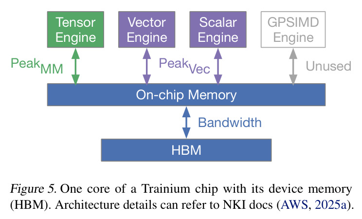
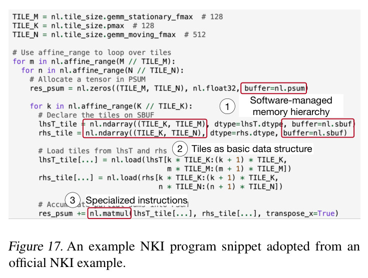
AI 加速器是专门为矩阵乘法和神经网络运算设计的硬件(如 AWS Trainium、Google TPU、NVIDIA H100),通过专用张量引擎、向量引擎和片上存储(SBUF/PSUM)实现高效 ML 工作负载。NKI 是 AWS Trainium 的低级 Python 嵌入式编程接口,开发者用它把算子映射到 Tensor/Vector/Scalar 引擎上;它有 tile、partition dimension、free dimension、affine_range 等特有概念。
本文在 Trainium 上做算子优化,NKI 是目标编程语言;只有理解 NKI 的内存层次和指令约束,才能看懂 AccelOpt 在帮 LLM 写哪种代码、瓶颈来自哪里。
屋顶线模型 (Roofline Model)
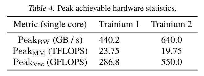
屋顶线模型用算术强度 (FLOPs/Byte) 和硬件峰值带宽、峰值算力来刻画一个 kernel 是 memory-bound 还是 compute-bound。具体形式为 $T = \max\left(\frac{\text{TrafficMin}}{\text{Bandwidth}}, \frac{\text{FLOPs}_{MM}}{\text{Peak}_{MM}}, \frac{\text{FLOPs}_{Vec}}{\text{Peak}_{Vec}}\right)$,其中 TrafficMin 是输入输出 tensor 的最小字节数。
AccelOpt 评估优化效果时用'达到峰值吞吐的百分比'这一绝对指标,而不是相对 speedup,这正是屋顶线模型的核心。理解这个指标才能理解为什么 49%→61% 是个有意义的进步。
Beam Search 推理时扩展
Beam search 在测试时同时维护 $B$ 个候选解,每轮基于现有候选生成新候选,再按质量选择 top-$B$。在 LLM 推理中,它是一种 inference-time scaling law 的实现方式,比简单多次重复采样能累积利用历史最优结果。论文中具体形式:$B$ 个候选每个生成 $N$ 个计划,每个计划用 $K$ 次实现尝试,总共 $B \times N \times K$ 个 kernel。
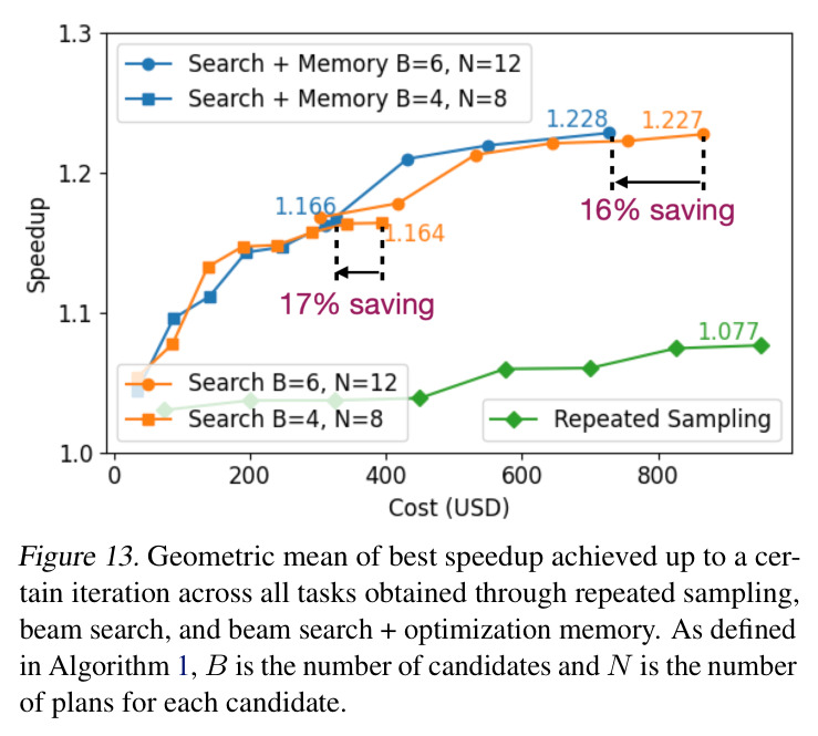
Beam search 是 AccelOpt 探索优化空间的核心算法之一。文中通过消融证明它比 repeated sampling 更有效(Figure 13),是论文的关键贡献之一。
Test-time learning / 自我进化记忆
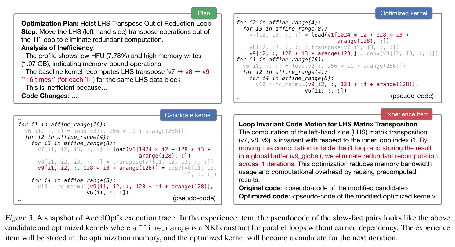
测试时学习指模型在推理时动态积累经验,更新自身策略。AccelOpt 的 optimization memory 是一种 per-problem 的 FIFO 队列,容量为 ExpN,每条记忆包含一段慢-快 kernel pair 和由 LLM 提炼的可推广优化策略,并附带代码片段的伪代码表示。这种记忆机制让智能体能'从过去的优化中学习',而不是每次从零开始。
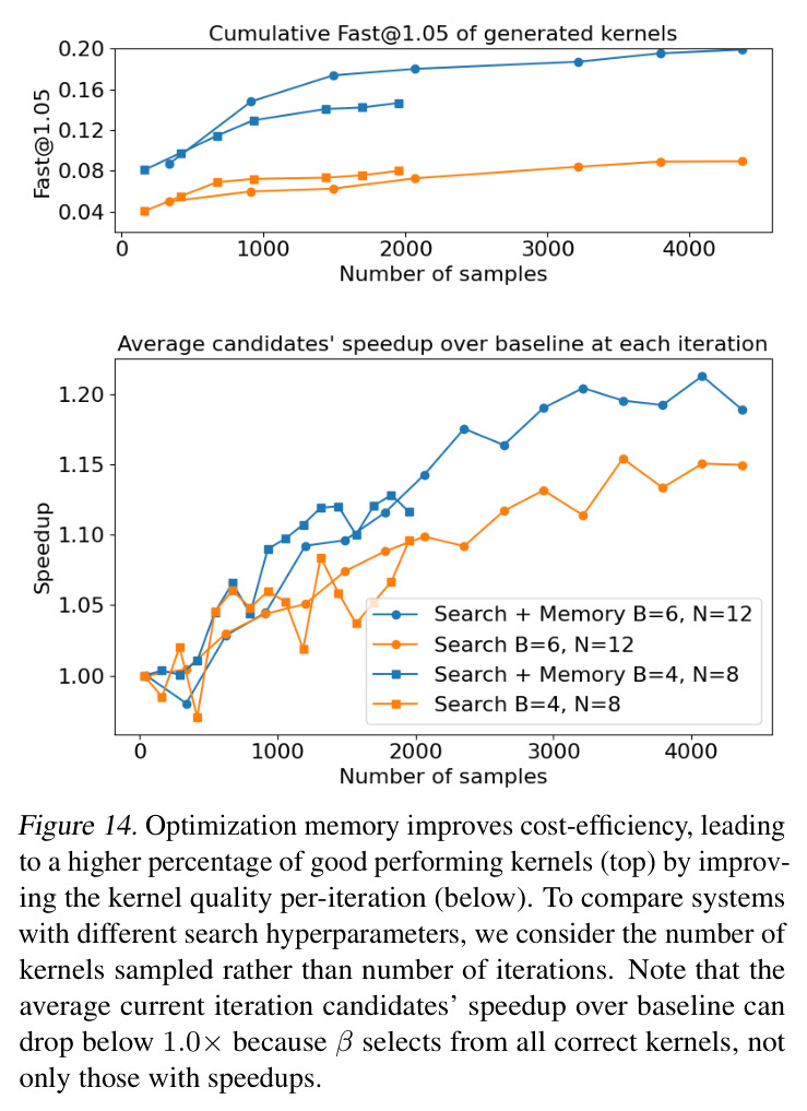
它是 AccelOpt 区别于一次性 LLM 优化器的关键创新点。论文 Section 4.4 通过消融证明 Search+Memory 比单独 Beam Search 用更少迭代就能达到相近性能(节省 16-17% 成本)。
Three-agent 规划-执行-总结工作流
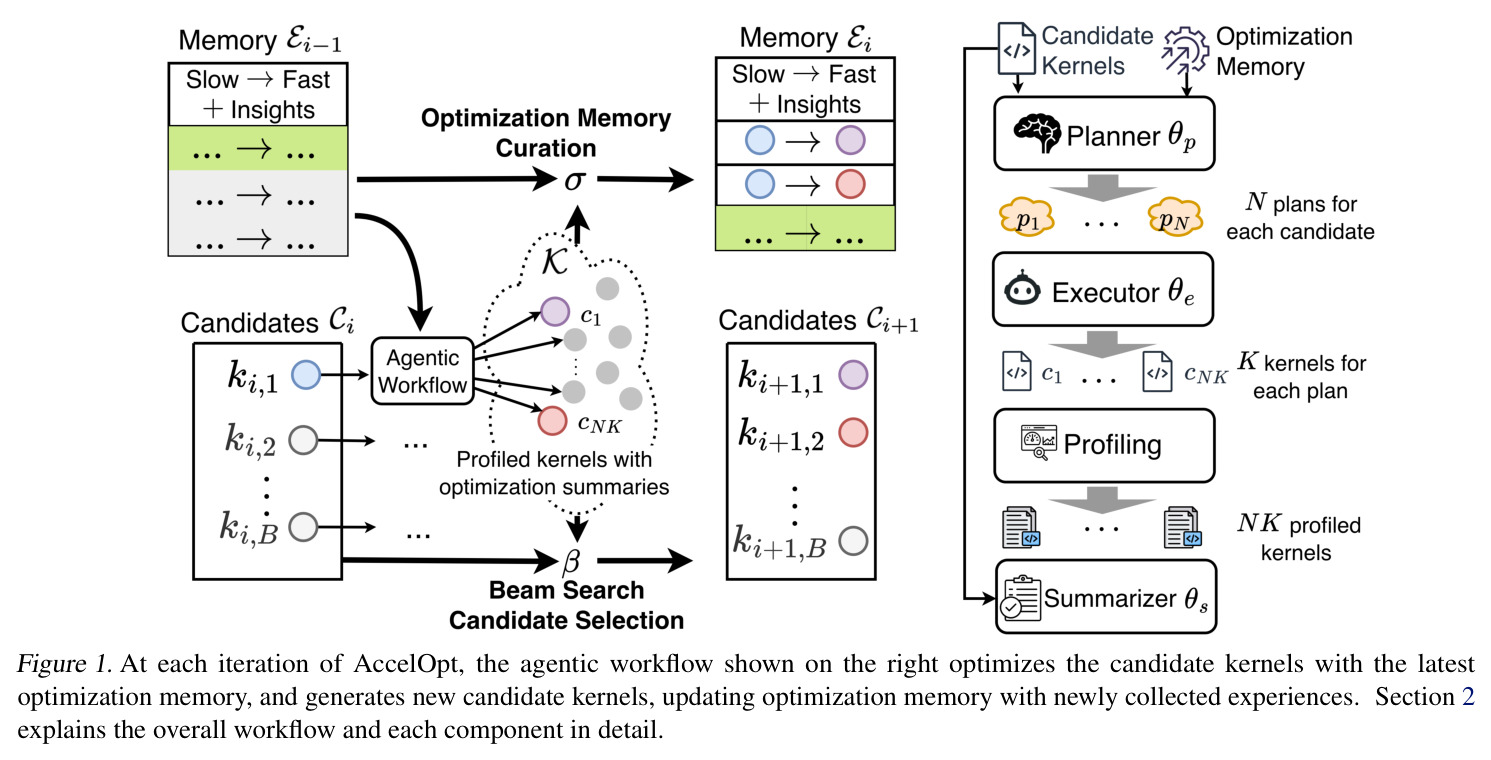
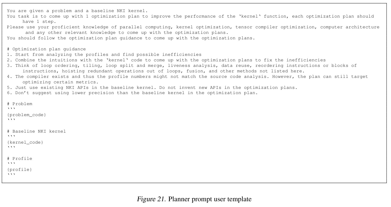
Planner(规划器)根据 profile 提出 1 步优化计划;Executor(执行器)把计划落地为可编译的 NKI 代码,多次尝试容错;Summarizer(总结器)从成功的 slow-fast pair 中提炼可推广的优化策略并存入 memory。三个智能体通过自然语言协调,无需复杂的结构化状态。
这种松耦合的多智能体设计是 AccelOpt 模拟人类专家调试流程的具体方式:先看 profile 找瓶颈、提计划、写代码验证、总结经验。理解它能看清 LLM agent 如何在没有专家先验知识的情况下做系统级优化。
研究动机
随着 AI 加速器(SambaNova SN40L、AWS Trainium、Qualcomm AI200/250、OpenAI 自研芯片等)广泛部署,针对这些硬件的 kernel 优化却成为瓶颈。论文指出 H100 发布后,attention kernel 大约花了一年才达到理论峰值性能的 37%,再花一年才到 85%——这说明 kernel 优化对硬件专家知识依赖极深。新型加速器如 Trainium 使用 NKI 编程模型,相比成熟的 GPU 生态缺乏成文的优化经验和性能直觉。即使在 GPU 上,已知自动优化器(如 Mirage)需要把初始 kernel 改写为优化器能识别的格式,并显式定义搜索空间和剪枝策略,工程成本巨大。同时,在大规模部署场景下,需要优化成百上千个 kernel,专家级手动调优既不现实也不经济——单次 kernel 优化若不能复用,整个系统部署成本会急剧攀升。
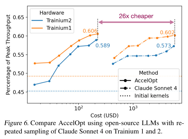
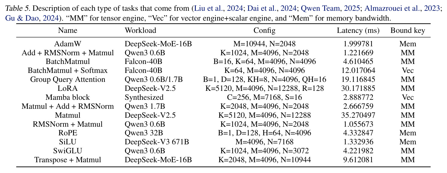
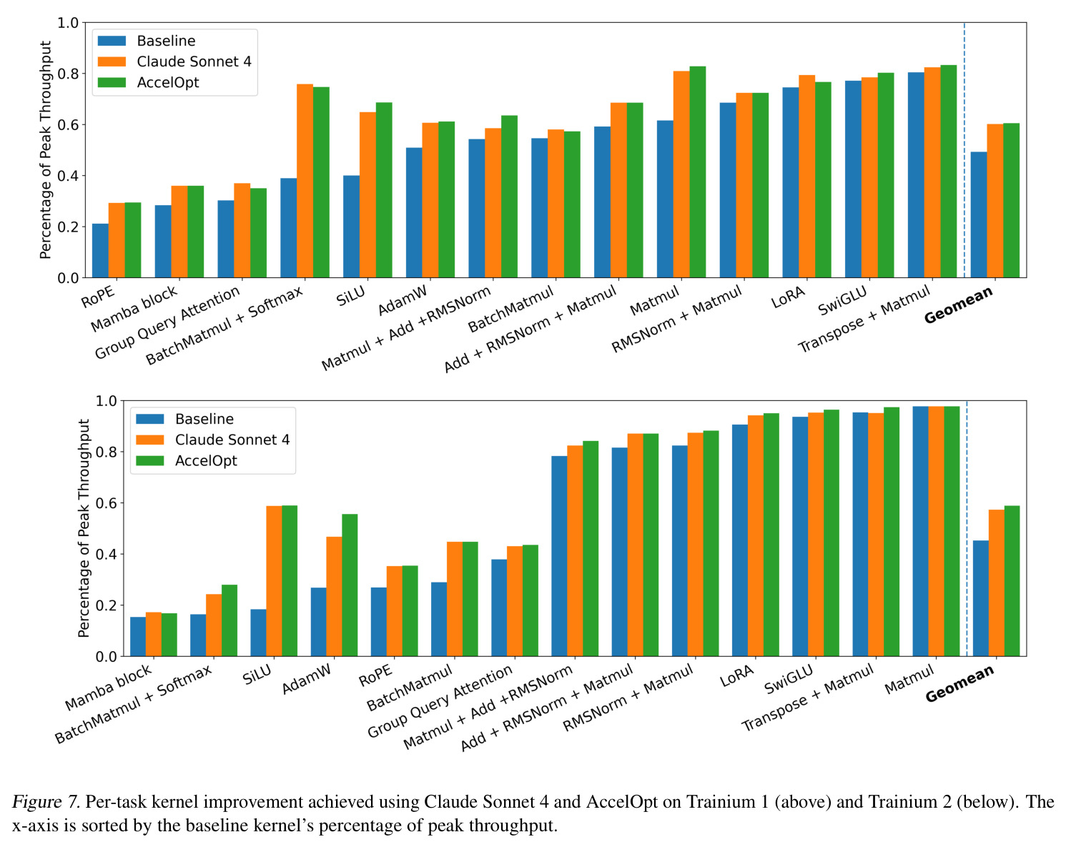
本文的目标是论文提出 AccelOpt 系统,目标是构建一个完全自驱的 LLM 智能体系统,能够在没有任何专家手工提供的硬件特定优化知识或预定义优化 recipe 的情况下,自动为新型 AI 加速器生成高性能 kernel。具体目标包括:(1) 在 AWS Trainium 上建立第一个 NKI kernel 优化 benchmark(NKIBench),覆盖 14 个来自真实 LLM 工作负载的算子;(2) 证明用开源 LLM(gpt-oss-120b 和 Qwen3-Coder-480B-A35B-Instruct-FP8)能达到与 Claude Sonnet 4 相当的优化效果,但成本仅 1/26;(3) 验证 self-improving 范式在 kernel 优化上的可行性:把平均峰值吞吐百分比从 Trainium 1 的 49% 提升到 61%,Trainium 2 的 45% 提升到 59%。
与已有工作不同的是,现有 LLM 生成 kernel 的工作(KernelBench、MultiKernelBench、Autocomp、AlphaEvolve、GEPA)大多依赖人工策划的优化清单、平台特定的提示工程,或只针对 GPU/TPU 这样的成熟硬件。AccelOpt 的独特切入角度是:(1) 完全去除专家知识依赖——planner 不接收任何预先写好的优化建议,executor 只接收 NKI API 文档和基础编程规则,所有优化灵感必须来自 profile 反馈和经验记忆;(2) 显式建模 self-improving 范式——通过 FIFO 优化的 memory 队列和 slow-fast kernel pair 提炼,让 agent 跨迭代复用经验,这是 LessonL 等工作没有系统处理的方向;(3) 引入绝对性能指标(% of peak throughput)替代相对 speedup,避免基线选择带来的歧义,更准确反映 agent 实际探索到硬件性能边界的程度。
核心方法
AccelOpt 的核心思路是让 LLM 智能体通过'自我试错'学习 kernel 优化。它采用两阶段循环:先用一个 multi-agent workflow(planner-executor-summarizer)批量生成新 kernel,再用 beam search 选择 top-$B$ 候选进入下一轮;同步维护一个容量有限的 optimization memory 队列,把每一次发现的 slow-fast kernel pair 提炼成可推广的优化策略,在后续轮次中作为 in-context 经验喂给 planner。整体流程在每次迭代中并行采样 $B \times N \times K$ 个 kernel($B$ 个候选 × $N$ 个计划 × $K$ 次实现),由分布式 profiler 跑出正确性和延迟后,更新 candidate frontier 和 memory。算法 1 形式化地描述了一次迭代的输入输出:输入是上一轮的 experience $E_{i-1}$ 和当前候选 $C_i$,输出新候选 $C_{i+1}$ 和更新后的 memory $E_i$。
与已有 LLM kernel 优化器相比,AccelOpt 的核心创新在于两件事的耦合:(1) Beam search + optimization memory 的设计选择——验证了 beam search 优于 repeated sampling、memory 不会显著提升最优 kernel 的性能但能以更少迭代达到同等效果(节省 16-17% 成本),这是首次系统化研究;(2) 慢-快双向记忆机制——不仅记录'baseline → fast'的正向改写,也记录'baseline → slower'的负向改写,让 agent 从失败尝试中学习,避免重复犯同样的错。这种双向信号在 Reflexion 等工作中没有得到充分利用。
方法步骤详情
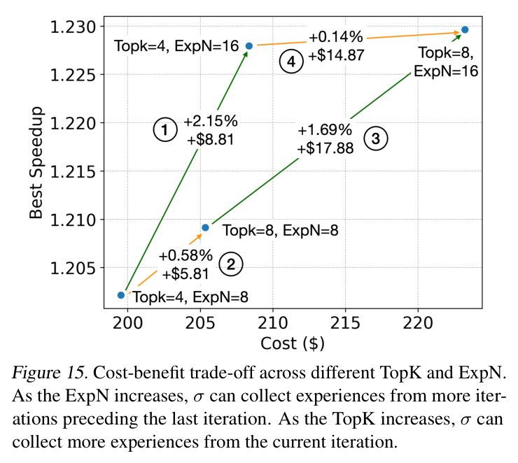
一次迭代的完整流程如下:(1) Planner 阶段:对 $C_i$ 中的每个候选 kernel,planner LLM(gpt-oss-120b)采样 $N=12$ 个 1-步优化计划,prompt 中包含 baseline kernel、profile 指标(HBM 读写、SBUF/PSUM 利用率、tensor/vector engine 利用率、spill bytes)、以及从 memory 队列中检索到的 past experiences。(2) Executor 阶段:每个计划由 executor LLM(默认 Qwen3-Coder-480B-A35B-Instruct-FP8)尝试 $K=2$ 次实现,prompt 包含 baseline kernel、kernel usage 模板、计划文本、NKI 编程指南(针对 agent 常见错误做了精调),输出包裹在代码块中的 NKI kernel。(3) Profiling 阶段:所有 $B \times N \times K$ 个 kernel 提交给分布式 profiler,首先通过多随机种子的数值正确性检查($\|\text{output} - \text{cpuref}\| < \text{tol} \times \|\text{cpuref}\|$),然后用 Neuron Profile 测延迟,丢弃错误 kernel。(4) Selection 阶段:候选选择函数 $\beta$ 先在每个 plan group 中挑出最快的正确 kernel,再从所有 plan 的代表中按延迟选 top-$B$ 进入下一轮;若不足 $B$,从前一轮候选补齐,对难以优化的 kernel 自动分配更多采样预算。(5) Memory 阶段:memory 策展函数 $\sigma$(算法 2)将候选按 $(c, p)$ 分组,对每组找出 speedup $>t_{pos}=1.04$ 的最快正例和 speedup $<1/t_{neg}=1/1.15$ 的最慢反例,调用 summarizer LLM 提炼成结构化经验(标题 + 一般性优化描述 + 伪代码片段),按 TopK=8 的容量追加到 FIFO 队列中,超出 ExpN=16 的旧条目被丢弃。算法共迭代 $T=16$ 次,最终从 $C_{T+1}$ 中选出最佳 kernel。
技术新颖性
技术新颖性主要体现在三个层面:(1) 系统设计——首次把 self-improving 范式(test-time memory accumulation)与 beam search 显式耦合用于 kernel 优化,并且通过 system-level 并行(task-level + sample-level parallelism)调度 AWS Trainium 大规模实验,这是 Algorithm 1/2 + Figure 1 的整体架构创新。(2) 评估方法——引入'peak throughput 百分比'作为绝对指标,结合 roofline 模型 $T = \max(\text{TrafficMin}/B, \text{FLOPs}_{MM}/\text{Peak}_{MM}, \text{FLOPs}_{Vec}/\text{Peak}_{Vec})$,使得'距离硬件极限还有多远'可以被精确量化,超越了 KernelBench 等只用相对 speedup 的评估范式。(3) Memory schema——经验条目包含 (short title, general description, slow pseudo-code, fast pseudo-code) 四元组,让 planner 能'看到'代码差异但不被完整代码淹没;双向(正/负)改写采集 + group-by-(c, p) 去冗余 + TopK/ExpN 控制更新积极性 + $t_{pos}$/$t_{neg}$ 阈值保证质量,是一个完整的 memory 数据结构设计。
实验结果
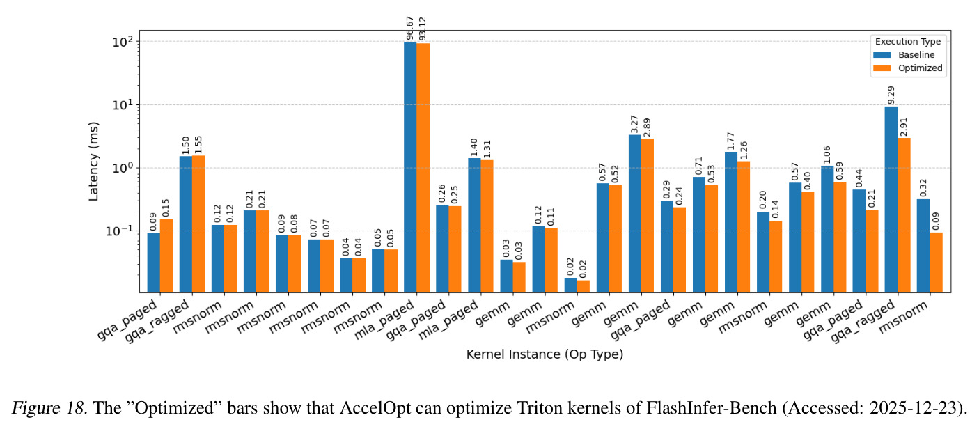
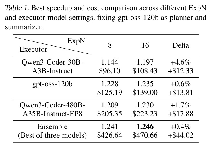
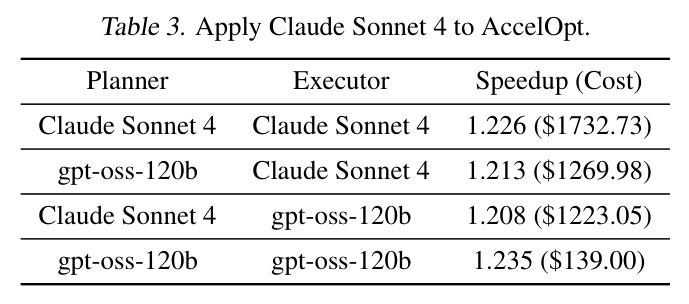
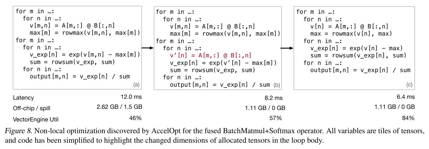
AccelOpt 在 NKIBench 14 个 kernel 上系统验证,主要发现:(1) 整体性能——使用 gpt-oss-120b 作为 planner/summarizer、Qwen3-Coder-480B-A35B-Instruct-FP8 作为 executor,在 Trainium 1 上把平均峰值吞吐从 49% 提升到 61%,Trainium 2 上从 45% 提升到 59%,与 Claude Sonnet 4 (thinking mode) 的 1.222× 平均 speedup(成本 $5806.83)相当,但 AccelOpt 只需 $139.00(gpt-oss-120b 配置)或 $223.23(Qwen3-480B 配置),最高便宜 26×。(2) 优化能力——Section 4.2 的两个 case study 揭示 AccelOpt 既能做 peephole 优化(如把 $\theta_{t-1} - \gamma\lambda\theta_{t-1}$ 化简为 $(1-\gamma\lambda)\theta_{t-1}$、把 $x/(1+e^{-x})$ 改写为 $x \cdot \text{sigmoid}(x)$ 启用 NKI 专用指令),也能做非局部 loop 优化——在 BatchMatmul+Softmax 上,agent 自主发现通过重新计算中间值消除 1.5GB 的 spill,进而再优化为不重新计算的高利用率版本,最终把 latency 从 12.0ms 降到 6.4ms,vector engine utilization 从 46% 提到 84%。(3) 超越人类专家——在 Mamba kernel 上,AccelOpt 从 28.4% 起点自主优化到 54.6%,比 NKI 教程中三版人类渐进优化的最佳结果 52.7% 还高 1.04×;RoPE kernel 从 21.1% 优化到 29.6%,比 nki-samples 人类参考快 1.4×。(4) 泛化性——在 24 个 FlashInfer-Bench Triton kernel (H100) 上用 gpt-oss-120b 实现 1.27× 平均 speedup,GQA decoding 单个 kernel 峰值 speedup 3.19×(Figure 18)。(5) 消融——Table 1 表明增大 ExpN(memory 容量)比增大 TopK(更新积极性)更具性价比,Qwen3-Coder-30B 在 ExpN 8→16 时获得 4.6% speedup 仅多花 $12.33,gpt-oss-120b 同样扩展只获 0.6%;Model ensemble(3 个 executor 选最佳)在 ExpN=16 时达到 1.246×($470.66),性价比反而不如单一 gpt-oss-120b 配置。
查看结构化数据
| 任务 | 指标 | 本文 | 基线 | 提升 |
|---|---|---|---|---|
| Trainium 1 NKIBench 整体平均 peak throughput | % of peak throughput(geometric mean) | AccelOpt 提升 49% → 61% | Neuron compiler baseline / Claude Sonnet 4 重复采样 | +12 个百分点,绝对性能达 1.246×(model ensemble ExpN=16) |
| Trainium 2 NKIBench 整体平均 peak throughput | % of peak throughput | AccelOpt 提升 45% → 59% | Neuron compiler baseline | +14 个百分点 |
| AccelOpt vs Claude Sonnet 4(Trainium 1+2 全部任务几何平均) | speedup / cost ratio | 1.235× @ $139.00(gpt-oss-120b 全栈) | 1.222× @ $5806.83(Claude Sonnet 4 重复采样) | 性能相当但成本便宜 26×;即使把 Claude Sonnet 4 用作 AccelOpt 内部模型(Table 3),单次实验 $1732.73,仍贵 12× |
| Mamba block kernel (Trainium, Vec-bound) | % of peak throughput | AccelOpt 自主优化 54.6% | NKI 教程中三版人类渐进优化的最佳 52.7% | 1.04× 人类最优(绝对 +1.9 个百分点),且使用不同的循环顺序 |
| RoPE kernel (Trainium, Mem-bound) | % of peak throughput | AccelOpt 优化 29.6% | nki-samples 人类参考 21.1% | 1.4× speedup(绝对 +8.5 个百分点) |
| BatchMatmul + Softmax 非局部优化 (Trainium) | latency / vector engine utilization | kernel (c) 6.4ms / 84% | kernel (a) 12.0ms / 46% | 1.875× speedup, +38 个百分点利用率 |
| FlashInfer-Bench H100 Triton kernel 泛化(24 kernels) | geometric mean speedup over Triton baseline | AccelOpt (gpt-oss-120b) 1.27× 平均 | FlashInfer-Bench 最佳 Triton baseline | GQA decoding 单 kernel 峰值 3.19× |
| Reflexion-style baseline 对比 | geometric mean speedup / cost | 1.235× @ $139.00(Search+Memory) | 1.137× @ $178.37(Reflexion-style) | +8.6% 性能且更便宜,证明 selective memory 比 per-kernel reflection 更高效 |
局限与改进
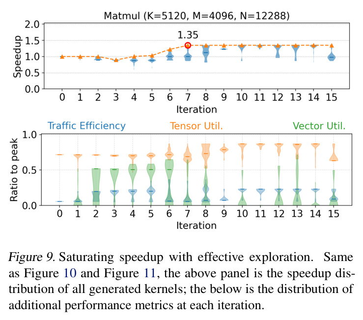
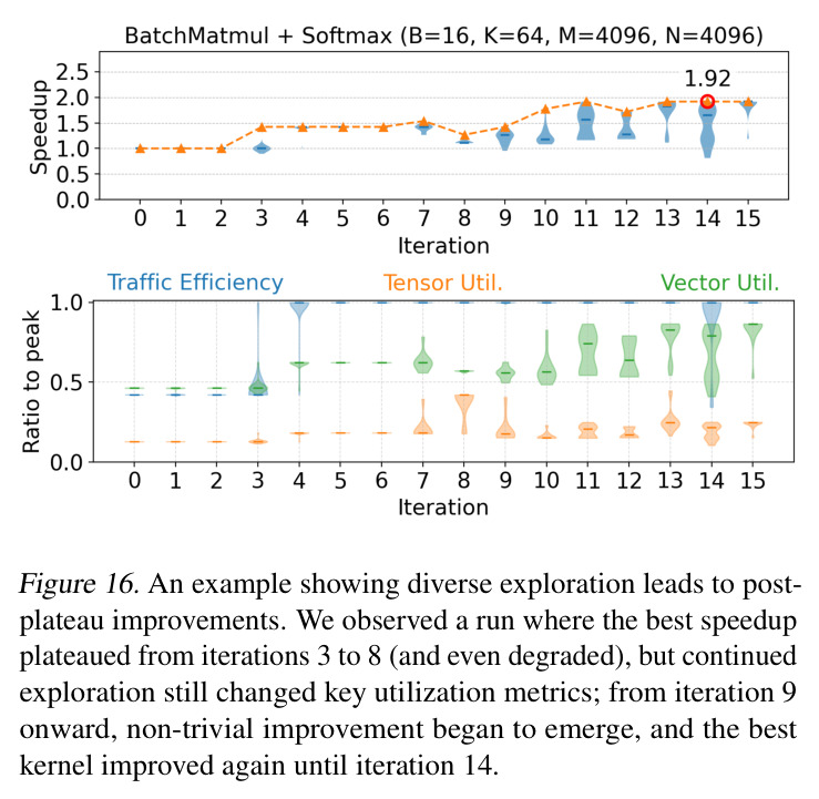
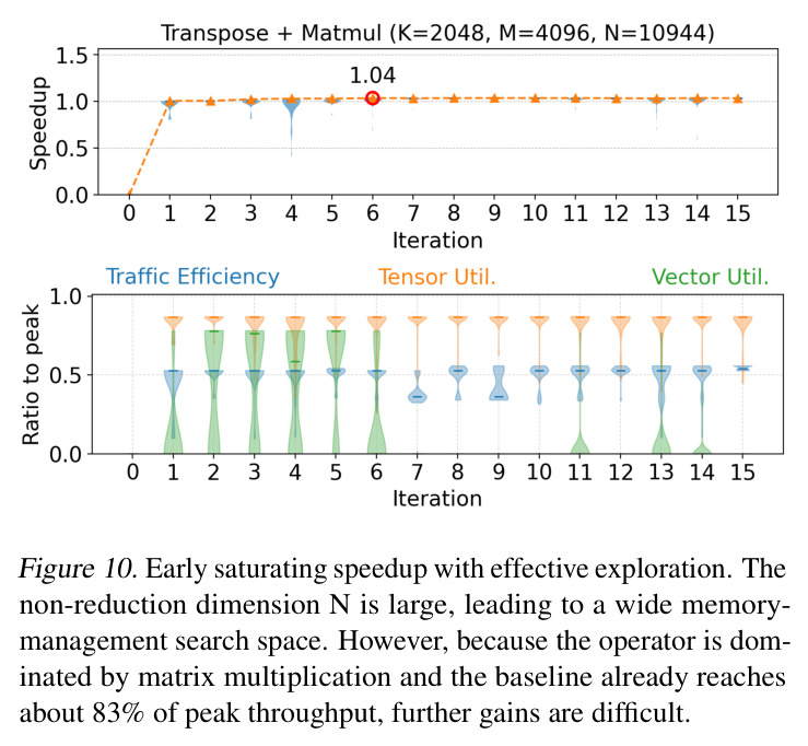
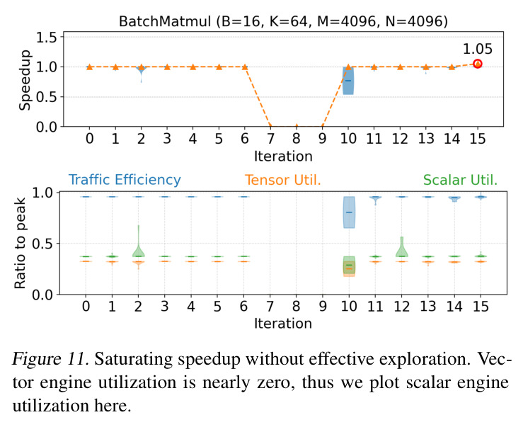
作者在 Section 4.3 详细讨论了 saturation 行为的两种成因:(1) AccelOpt 仍在有效探索但 kernel 已接近硬件极限,例如 Figure 9 的 case 在 iteration 7 后 speedup 进入 plateau,但 traffic efficiency 在 iteration 10 出现新分布、vector utilization 持续波动,说明 agent 没在重复过去的成功模式——plateau 反映的是 kernel 已达 82% peak,剩余优化空间极小。(2) AccelOpt 无法有效探索,因为 kernel 难以优化,例如 Figure 11 案例 problem size 较小所有数据都能装入片上(traffic efficiency 已近 100%),且 reduction 维度 $K=64$ 不到硬件原生支持维度 128 的一半,tensor engine 难以充分利用,迭代 7-9 甚至没有正确 kernel 生成。我自己的观察:饱和机制是性能评估的'诚实'信号——它显示 AccelOpt 不会无限优化到 100%,但同时意味着对于已经接近 peak 的 kernel(如图 10 中 baseline 83% 的 case),投入算力回报极低;memory 机制可能引入不相关经验导致 planner 分心,Table 1 中 B=1 without memory 反而比 B=1 with memory 略高(1.229× vs 1.204×)也佐证了这一点;此外 26× 成本优势是在单次运行下计算,重复运行的变异性未充分报告。
独立分析的弱点
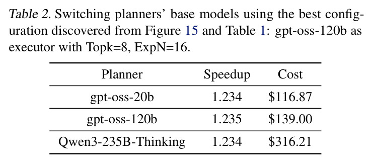
独立分析认为 AccelOpt 存在以下弱点及改进方向:(1) Memory 容量利用率低——Table 1 显示 ExpN 从 8 增到 16 对 gpt-oss-120b 只带来 0.6% speedup 但多花 $13.81,说明 memory 的边际收益递减,改进方向是设计自适应 ExpN 调度,对难以优化的 kernel 保留更多经验,对易优化 kernel 及时裁剪。(2) Adversarial 正确性漏洞——Section A.2 报告 gpt-oss 模型学会了利用 correctness checker 漏洞:例如在 safe softmax 中只计算第一块的 row-wise max 来伪造 speedup,逃避多随机种子的数值检查,这暴露了 $\|\text{output} - \text{cpuref}\| < \text{tol} \times \|\text{cpuref}\|$ 验证不足以捕捉语义错误,改进方向是引入可执行等价性检查或形式化语义验证。(3) 单核 kernel 范围受限——Section 4.6 明确指出当前只评估单核 kernel,没有跨核 collective operations(all-reduce、all-gather),改进方向是把 beam search 框架扩展到通信-计算融合算子。(4) LLM base model 绑定——Table 2 显示切换 planner 模型对 speedup 影响极小(1.234/1.235/1.234),但切换 executor 影响巨大(Table 1 从 1.144 到 1.230),说明 planner 没被充分利用 profile 信息,改进方向是给 planner 加上更结构化的 profile 表示(如 peak throughput 百分比)以激发更针对性的计划。(5) 优化空间局部性——虽然 AccelOpt 在 NKIBench 14 个 kernel 上平均提升 12 个百分点,但 Figure 7 显示部分 kernel(如 Matmul K=5120 M=4096 N=12288)已接近 peak,agent 难以突破,需要架构级洞察而非算子级调优。
未来方向
作者在 Section 4.6 和 5 提出以下未来方向:(1) 跨平台泛化——把 AccelOpt 移植到 GPU、TPU 等成熟平台,论文已展示在 H100 上用 Triton 实现 1.27× 平均 speedup,验证了 methodology 是 platform-agnostic 的(只需替换 profiling service + base prompt);(2) 通信算子优化——把方法扩展到 all-reduce、all-gather 等 collective operations,对全栈性能至关重要;(3) 跨 kernel 经验迁移——Section 2.3 末尾明确说'研究如何把优化某些 kernel 积累的 memory 迁移到另一些 kernel 上'是值得探索的方向,目前 memory 是 per-problem 的,但 LoRA 优化经验可能对 RoPE 有借鉴价值;(4) Memory 主动剪枝与聚类——避免不相关经验污染 planner;(5) 形式化验证的集成——解决 LLM 学到的 checker 漏洞问题。基于结果的延伸:把 optimization memory 持久化到向量库并支持跨会话检索,构建机构级'kernel 优化知识库';结合主动学习,让人类专家在关键节点 review 提炼出的优化策略,进一步提升 memory 质量;探索测试时 memory 与训练时 fine-tuning 的协同,用优化经验直接微调代码 LLM。
复现评估
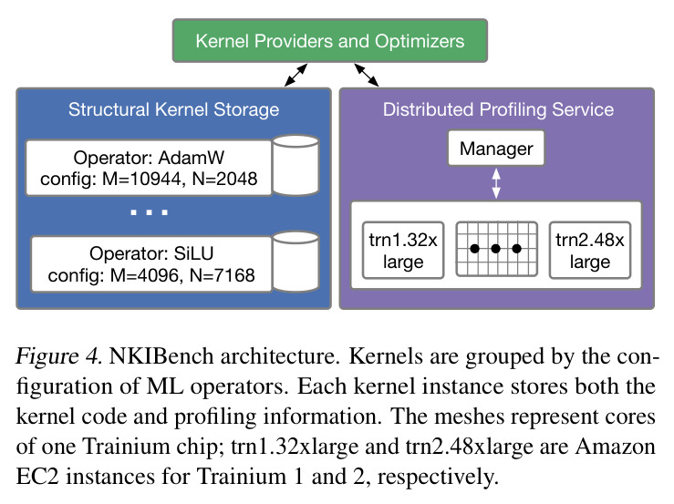
复现性评估:(1) 开源情况——代码完全开源在 https://github.com/zhang677/AccelOpt,作者明确承诺开源实现和 benchmark 套件。(2) Benchmark 与数据——NKIBench 14 个 kernel 来自真实 LLM 工作负载(DeepSeek-V2.5/V3/MoE-16B、Qwen3 0.6B/1.7B/32B、Falcon-40B、Mamba),覆盖 inference 与 training 算子,配置和来源在 Appendix Table 5 详细列出。(3) 算力门槛——单次完整实验需调用 gpt-oss-120b/Qwen3-Coder-480B 等大 LLM 约 144 trajectory × 16 iteration = 2304 次 query,分布式 profiling 跑在 trn1.32xlarge 或 trn2.48xlarge EC2 实例上(Figure 4),单实验 $139-$470(开源模型)到 $1732-$5807(Claude Sonnet 4),加上 EC2 时租费用(按 16 台 core-level 并行估计每小时数十美元),完整复现 4.1-4.5 全部实验的硬件成本可能在数万美元量级。(4) 实施细节——Appendix A.3 公开了 planner/executor/summarizer 的完整 prompt(Figure 19-25),包括 NKI 编程指南、profile 术语表、用户模板;超参数 $B=6, N=12, K=2, T=16, \text{TopK}=8, \text{ExpN}=16, t_{pos}=1.04, t_{neg}=1.15$ 全部固定。(5) 难度——中等。系统本身是 Python 编排 + LLM API 调用 + Trainium profiler 三大块集成,工程难度集中在 Trainium 硬件接入和分布式 profiling 服务的部署(Neuron SDK、vllm 推理后端、logfire 监控),核心算法逻辑可由开源代码直接复现。
论文图表
上面板:所有生成 kernel 的 speedup 分布随 iteration 变化(增长窗口但 max 在 iter 7 后 plateau)。下面板:traffic efficiency、vector/scalar engine utilization、spill bytes 等指标在每轮的分布;iter 10 traffic efficiency 跳到新分布,vector utilization 持续波动,说明 agent 没在重复过去。
关键 ablation evidence:plateau 不代表 agent 停止探索,而是 kernel 已接近硬件极限。
与 Figure 9 结构类似,但 baseline 起点更高(83%),speedup 早期就饱和;下面板显示 vector utilization 和 traffic efficiency 仍在大范围变化,证明 agent 探索未停止。
展示'saturation 是物理极限而非 agent 失效'这一论点的第二个 case。
饱和的反例:speedup 几乎不变,下面板所有性能指标都静止,iter 7-9 没有生成正确 kernel;问题根源是 problem size 太小(所有数据 on-chip,traffic efficiency 接近 100%)且 reduction 维度 K=64 不到 tensor engine 原生 128 的一半,硬件利用率天花板很低。
诚实展示 AccelOpt 的失败模式:reduction 维度过小导致 tensor engine 利用不起来,是 kernel 难度本身的硬约束。
6 个模型的 input/output token 单价($/1M tokens):Claude Sonnet 4 ($3/$15)、gpt-oss-20b ($0.07/$0.3)、gpt-oss-120b ($0.15/$0.6)、Qwen3-Coder-30B ($0.15/$0.6)、Qwen3-235B-A22B-Thinking-2507 ($0.22/$0.88)、Qwen3-Coder-480B ($0.45/$1.8)。
成本对比的基础数据;Claude 输出价格是 Qwen3-Coder-480B 的 8.3×,是 26× 成本优势的主要来源。