面向无数据扩散蒸馏的一致分布匹配 Consistent Distribution Matching for Data-Free Diffusion Distillation
单一学生网络统一生成与速度估计,实现无数据、免模拟的少步扩散蒸馏
前置知识
流匹配(Flow Matching, FM)
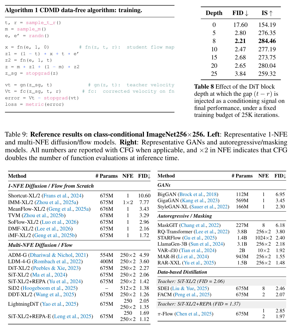
一类连续归一化流生成范式:定义affine插值路径 $x_t=\alpha_t x_0+\sigma_t x_1$(线性调度下条件速度恒为 $v_t=x_1-x_0$),训练网络 $v_\theta(x_t,t)$ 用条件流匹配目标 $\mathcal{L}_{CFM}=\mathbb{E}\|v_\theta(x_t,t)-v_t(x_t|x_0,x_1)\|_2^2$ 回归边缘速度场;推理时数值积分ODE $dx_t/dt=v_\theta$,通常需要上百次前向评估(如SiT-XL/2为 $250\times2$ NFE)。
本文的教师就是流匹配模型,蒸馏的本质是把这个昂贵的积分过程压缩进一个少步学生网络,所有推导都在FM的速度场语言下进行。
流映射与平均速度(Flow Map & Average Velocity)
流映射 $f(x_t,t,r)$ 把ODE轨迹上 $t$ 时刻的状态直接跳到 $r$ 时刻;平均速度定义为 $u(x_t,t,r):=\frac{x_t-x_r}{t-r}=\frac{1}{t-r}\int_r^t v(x_\tau,\tau)\,d\tau$,并约定 $u(x_t,t,t):=v(x_t,t)$。对恒等式 $\int_r^t v\,d\tau=(t-r)u$ 两端对 $t$ 求全导数得关键恒等式 $v=u+(t-r)\frac{d}{dt}u$(MeanFlow的核心量)。
CDMD学生网络的参数化就是 $u_\theta(x_t,t,r)$:它既能一步生成 $G_\theta(z)=z-u_\theta(z,1,0)$,又能借上述恒等式给出自身瞬时速度的代理,是全文的核心对象。
分布匹配蒸馏(DMD)与 fake score 网络
DMD把学生分布 $q_t$ 与教师分布 $p_t$ 的反向KL作为生成器损失,梯度形如 $\nabla_\theta\mathcal{L}_{SD}\approx\mathbb{E}\,w_t(s_{fake}-s_{real})^\top\frac{\partial G_\theta}{\partial\theta}$。其中教师score $s_{real}$ 冻结,而 $s_{fake}\approx\nabla_x\log q_t$ 必须由第三个辅助网络在学生生成样本上持续训练,形成类似GAN的双玩家优化,且该网络推理时被丢弃。
CDMD的出发点正是消除这个第三网络:论文把KL/Fisher散度改写成速度形式后,$v_{fake}$ 由学生网络自身导出,这是方法成立的根基,也是与DMD2/SiD/FreeFlow对比的坐标系。
Fisher 散度及其速度形式
Fisher散度 $D_F(q_t\|p_t)=\mathbb{E}_{\hat{x}\sim q_t}\|\nabla_{\hat{x}}\log q_t(\hat{x})-\nabla_{\hat{x}}\log p_t(\hat{x})\|^2$ 度量两个score场之差。论文证明在线性调度下score差与速度差仅差时间标量因子,于是分布匹配可等价写成 $\mathcal{L}_{VD}=\mathbb{E}\,\bar{w}_t\|v_{fake}(\hat{x}_t,t)-v_{real}(\hat{x}_t,t)\|_2^2$,$\bar{w}_t=(1-t)^2t^{-2}w_t$。
CDMD的损失就是Fisher散度的速度形式:只要能在学生状态上估计 $v_{fake}$,就能用教师速度 $v_{real}$ 做回归目标,这决定了整个目标函数的设计。
JVP(Jacobian-Vector Product,前向模式自动微分)
JVP一次前向计算向量-雅可比积 $\mathrm{JVP}(f;\dot{x})=Df\cdot\dot{x}$,无需构造完整雅可比矩阵,开销约等于一次额外前向。在本文中用于计算总导数 $\frac{d}{dt}u_\theta=\mathrm{JVP}(u_\theta;(\frac{d\hat{x}_t}{dt},1,0))$,切向的 $1$ 对应 $\partial_t$ 分量、$0$ 对应 $r$ 固定。
速度代理中的修正项 $(t-r)\frac{d}{dt}u_\theta$ 靠JVP实现;论文用专门一章分析该JVP在无数据情形下的方差并证明应选教师速度作切向,是训练稳定性的关键,也需要定制Flash-Attention内核支持。
Classifier-Free Guidance(CFG)
引导生成技术:$v_{cfg}(x_t,t|c)=(1-w)v(x_t,t|\varnothing)+w\,v(x_t,t|c)$,通过外推条件与无条件预测提升样本质量与条件吻合度;推理时每步需条件/无条件两次评估(NFE翻倍),且引导会改变教师实际访问的概率路径。
CDMD蒸馏的是引导后的教师动力学:学生以 $w$ 为额外条件($w\sim U[1,2]$)、目标用 $v_{cfg++}$;论文还发现引导强度 $w$ 直接决定多步推理是增益还是退化,是重要消融对象。
研究动机
扩散与流模型生成一张图需数值求解ODE,动辄数百次前向评估(如SiT-XL/2需 $250\times2$ NFE才达FID 2.06),推理缓慢。现有蒸馏管线有三大负担:其一,多数方法(DMD2、SiD、MeanFlow、FACM等)依赖外部蒸馏数据,对真实样本加噪构造中间训练状态,但这些数据往往不同于教师训练数据——当教师经过微调、使用classifier-free guidance/autoguidance或在专有数据上训练时,加噪真实数据得到的状态会系统性偏离教师生成时实际经过的概率路径 $p_t$,学生被"错位"状态监督;其二,直接在教师轨迹上监督需要反向模拟(如BOOT),开销大;其三,DMD/SiD/FreeFlow/CTM还需第三个辅助网络(fake score模型或判别器)与第二个优化器,双玩家优化难训练,fake score模型要被高频更新以跟踪生成器分布,消耗大量训练算力却在推理时丢弃。Figure 1显示iCT-XL训练需33GB、IMM-XL需37GB显存,而本方法只需20GB,训练负担直接限制可扩展性。
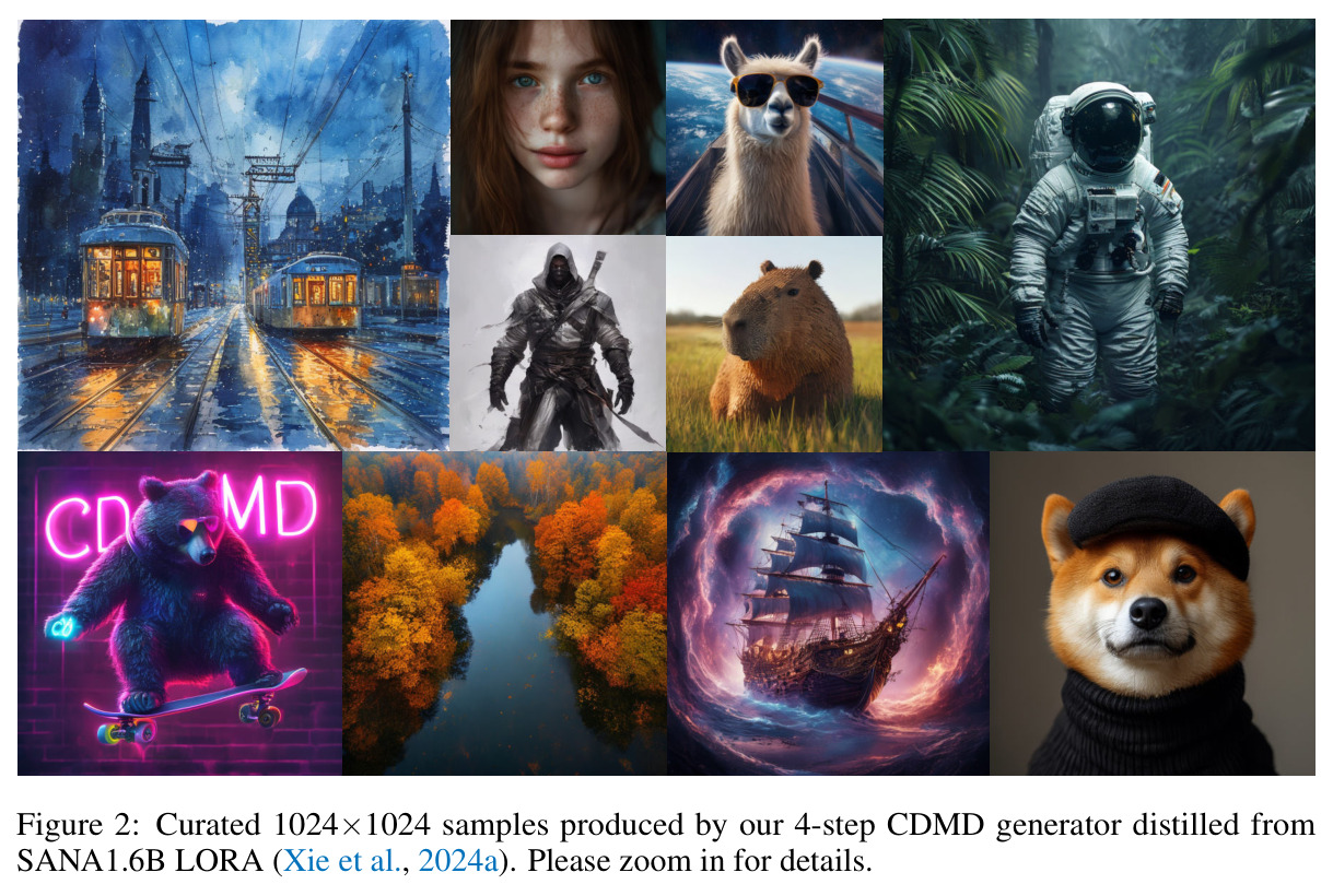
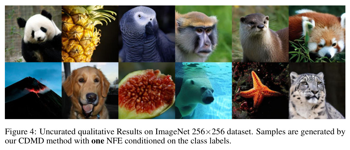
本文的目标是本文要回答一个核心问题:能否在不依赖外部蒸馏数据、不做教师rollout模拟、不引入辅助fake score网络的前提下,把一个强大的扩散/流教师蒸馏成1-4步的高质量学生?设定上训练时只允许"冻结教师+可训练学生"两个网络、一个损失函数、一个优化器,训练状态全部由学生自举(bootstrap)加解析前向加噪构造;同时希望学生的流映射参数化保留推理时在1、2、4步之间灵活伸缩的能力。量化目标是在ImageNet 256×256类条件生成上取得数据免费蒸馏的SOTA(最终1-NFE FID 2.04),4-NFE逼近教师水平(1.37 vs 教师的1.35),在SANA-1.6B文生图上验证可扩展性,并给出训练目标收敛的理论保证与唯一最优解的刻画。
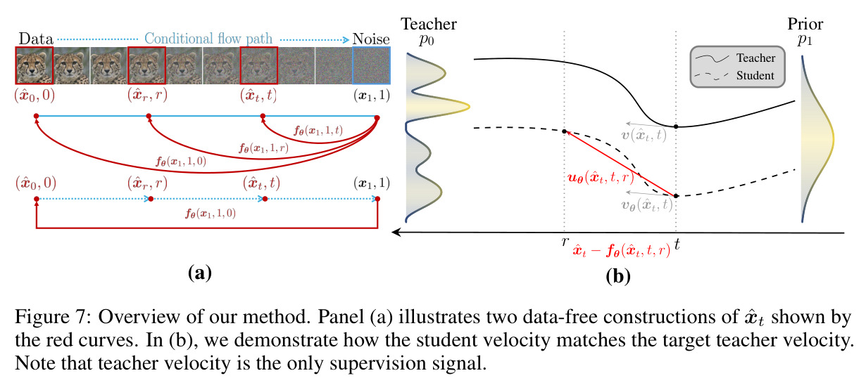
与已有工作不同的是,本文的独特切入是用一个网络同时承担"生成器"和"自身速度代理"两个角色,从而消掉第三网络。作者从Fisher散度的速度形式出发:匹配学生与教师分布等价于在共同状态上匹配二者的速度场 $v_{fake}$ 与 $v_{real}$;他们不再另训网络估计 $v_{fake}$,而是利用流映射的平均速度恒等式 $v=u+(t-r)\frac{d}{dt}u$,让学生网络 $u_\theta(x_t,t,r)$ 自己给出速度代理。与FreeFlow的"先验锚定"(只能从 $t=1$ 出发、还需LoRA代理模型做VSD修正)不同,CDMD在任意子区间 $[r,t]$ 上施加监督、天然支持多步推理伸缩;与MeanFlow/CM/FACM依赖真实数据构造状态不同,CDMD的状态由学生rollout加解析加噪得到。理论上还证明了最小化局部一致性残差蕴含学生推前分布按时间平均的 $\mathcal{W}_2$ 距离收敛到教师边缘分布,且全局最优解唯一恢复教师平均速度场——为"学生自举状态替代教师轨迹"提供了原理性辩护。
核心方法
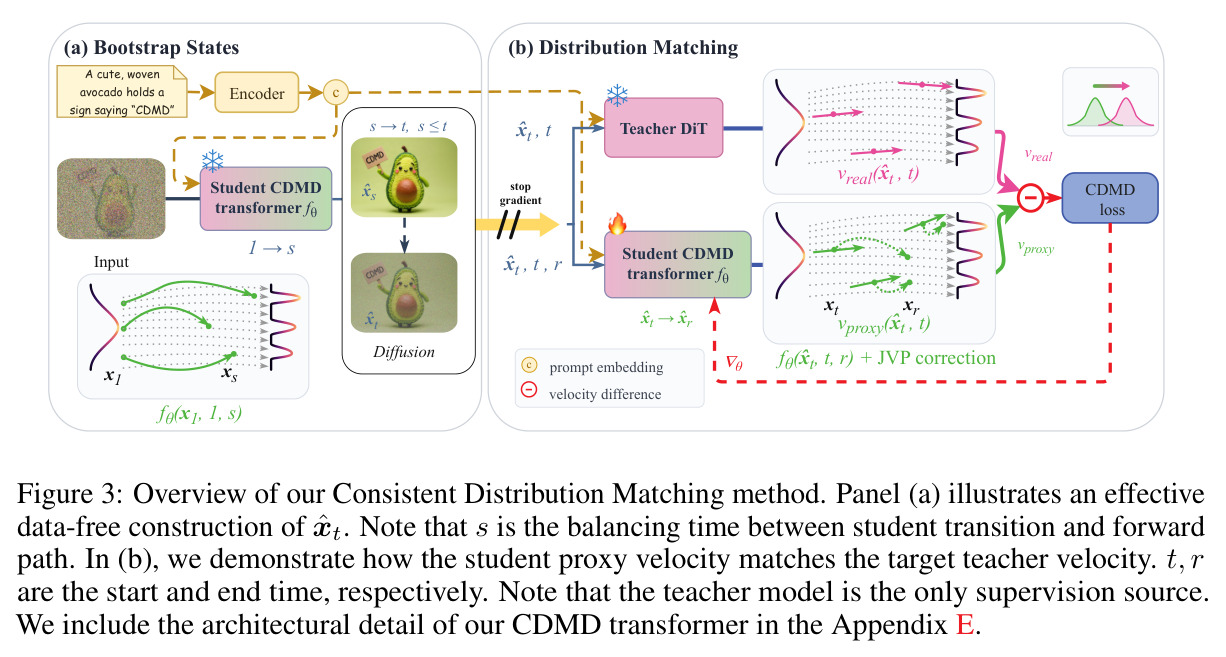
直觉上,DMD类方法要训练第三方网络"跟踪"学生分布,代价高昂;CDMD让学生"既会画、又能说出自己怎么画":流映射网络 $u_\theta(x_t,t,r)$ 输出任意区间 $[t,r]$ 的平均速度,一步生成 $G_\theta(z)=z-u_\theta(z,1,0)$,瞬时速度代理由恒等式 $v_\theta=u_\theta+(t-r)\frac{d}{dt}u_\theta$ 给出,总导数用一次前向模式JVP计算。技术路线:(1) 从先验采 $z$,经学生去噪到更早时刻 $s$、再按闭式路径加噪回 $t$,构造 $\hat{x}_t=\frac{1-t}{1-s}f_\theta(z,1,s)+\frac{t-s}{1-s}\varepsilon$($s=0$ 为加噪的一步样本、$s=t$ 为学生路径状态,按 $m$ 混合);(2) 冻结教师在 $\hat{x}_t$ 给出监督速度 $v(\hat{x}_t,t)$(引导时用 $v_{cfg++}$);(3) 以教师速度为切向算detach的JVP修正项;(4) 最小化二者MSE(式(7))。推理用 $f_\theta(x_t,t,r)=x_t-(t-r)u_\theta$ 做1-4步采样,全程无真实数据、无教师模拟。
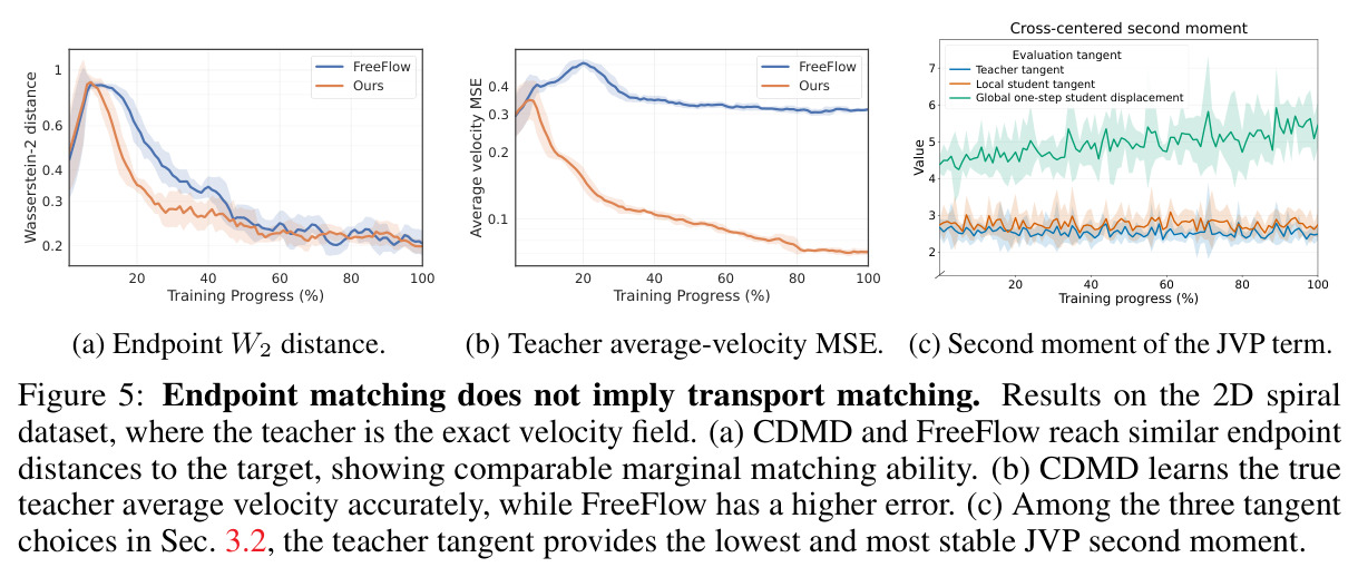
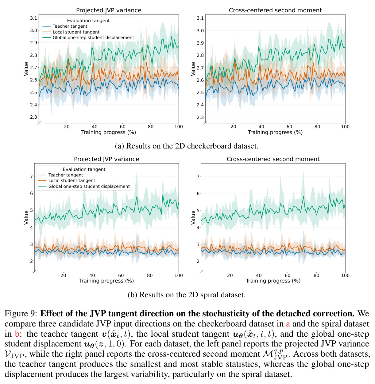
核心创新是把"分布匹配"与"局部传输一致性"统一进一个两模型目标。区别于DMD/SiD/FreeFlow:不需要辅助fake score/代理网络——Fisher散度的速度形式 $\mathcal{L}=\mathbb{E}\,\bar{w}_t\|v_{fake}-v_{real}\|_2^2$ 中,$v_{fake}$ 由学生网络自身经 $v=u+(t-r)\frac{d}{dt}u$ 导出,双玩家优化退化为单目标回归;区别于MeanFlow/CM/FACM:不需要真实数据构造训练状态——自举状态 $\hat{x}_t$ 虽不在教师路径上,但目标会把学生概率路径 $q_\theta^t$ 逐步拉向教师路径 $p_t$,教师因此在"与学生动力学相关的状态"上纠错,且状态越噪越接近教师训练分布、监督越可靠;区别于FreeFlow的先验锚定:CDMD学任意区间 $[t,r]$ 的平均速度,保留多步伸缩能力。另一关键设计是以教师速度 $v(\hat{x}_t,t)$ 作JVP切向——论文用二阶矩分解 $M^{JVP}_{q,p}=V^{JVP}_q+\|\mu_q-\mu_p\|^2$ 证明其方差最小最稳(Fig. 5c、Fig. 9),首次量化诊断了此类训练的不稳定来源。
方法步骤详情
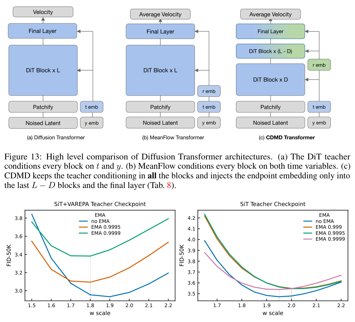
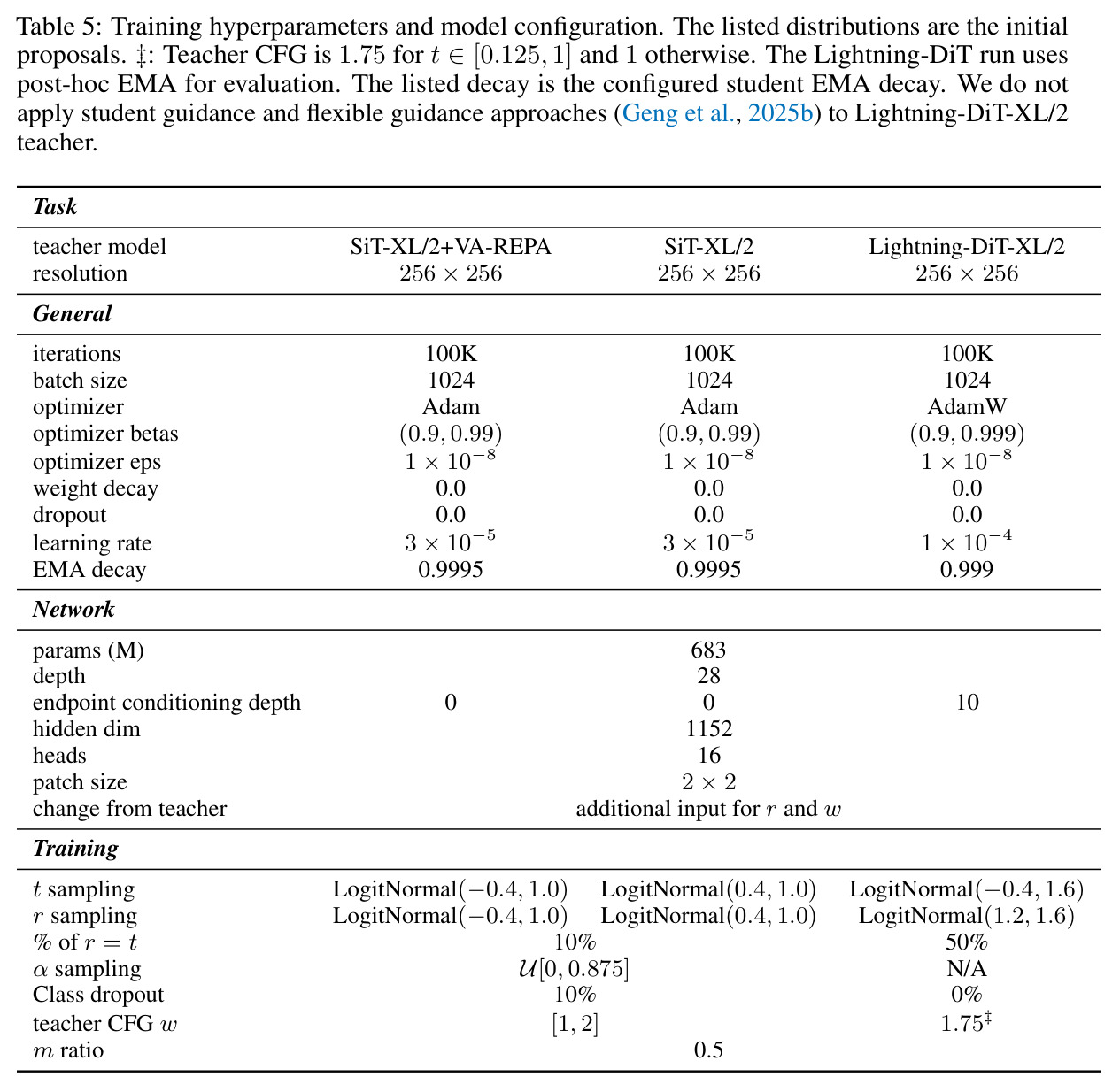
训练流程(Algorithm 1):(1) 从LogitNormal采 $t,r$($0\le r\le t<1$),按比例混入 $t=r$ 对(SiT教师10%、LightningDiT教师50%),采混合率 $m$。(2) 构造状态:采 $z$,一次学生前向得 $\hat{x}_0=f_\theta(z,1,0)$;$s=0$ 分支 $z_1=(1-t)\hat{x}_0+t\varepsilon'$,$s=t$ 分支 $z_2=f_\theta(z,1,t)$;按 $z=mz_1+(1-m)z_2$ 混合并stop-gradient——每步仅一次学生评估。(3) 教师监督:冻结教师输出 $v(\hat{x}_t,t)$;SiT教师以 $w\sim U[1,2]$ 采样并嵌入学生条件,LightningDiT固定1.75,文生图目标用 $v_{cfg++}$。(4) 学生修正速度:JVP以切向 $(v(\hat{x}_t,t),1,0)$ 算 $\frac{d}{dt}u_\theta$ 并detach,得 $v_\theta=u_\theta+(t-r)\cdot\mathrm{sg}[\frac{d}{dt}u_\theta]$。(5) 最小化 $\|v_\theta-v\|_2^2$(Adam/AdamW,100K迭代,batch 1024)。(6) 采样:$f_\theta(x_t,t,r)=x_t-(t-r)u_\theta$,从 $t=1$ 用Euler/DDIM走1-4步;架构上28块DiT新增 $r$、$w$ 嵌入,端点条件仅从第10块起注入。
技术新颖性
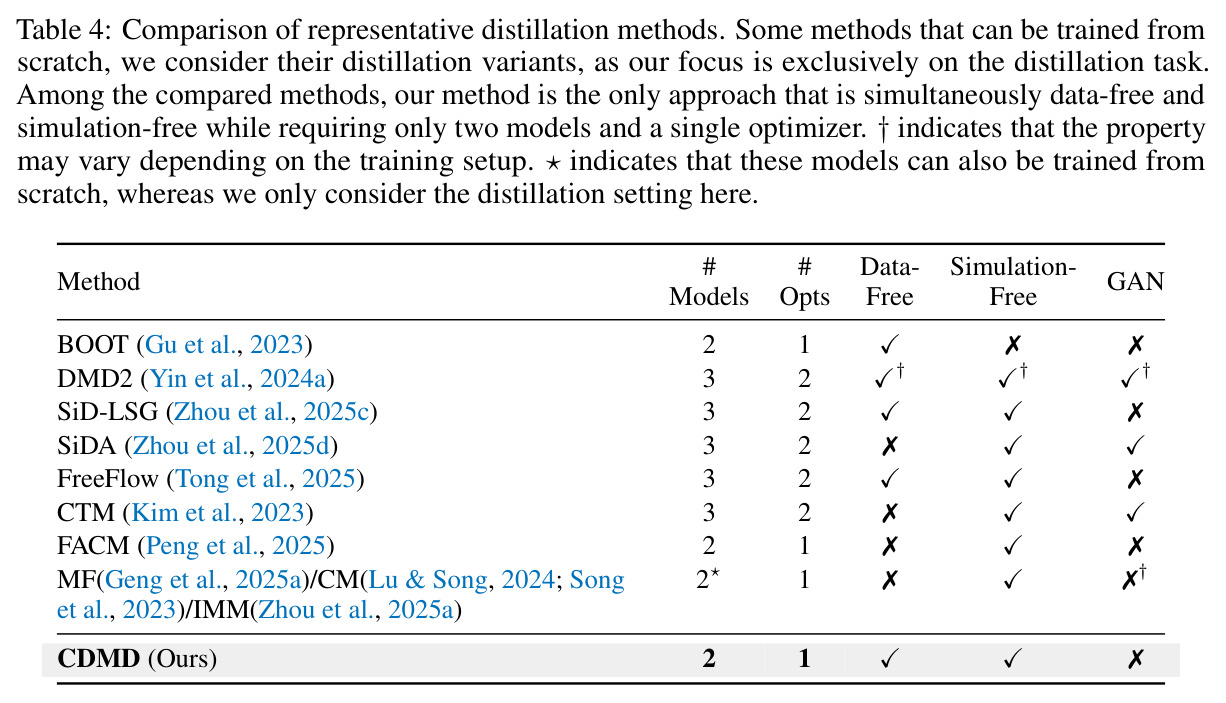
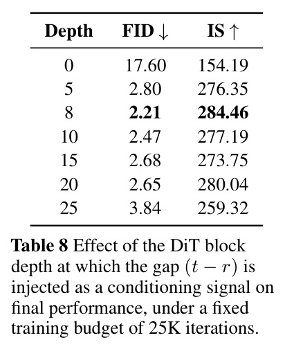
新颖性四点。第一,极简架构:Table 4显示CDMD是唯一同时"无数据+免模拟+2网络+1优化器+无GAN"的方法(DMD2/SiD/FreeFlow/CTM需3网络2优化器,BOOT需模拟,FACM/MeanFlow/CM需真实数据)。第二,理论:定理3.1证明(a)在连续性与一致可积条件下 $\mathcal{L}_{CDMD}\to0$ 蕴含 $\int\mathcal{W}_2^2((f_\theta(\cdot,1,r))_\#p_1,p_r)\nu(dr)\to0$,且不要求监督状态采自教师路径;(b)全局最优解几乎必然恢复教师平均速度 $u$,即目标可识别;证明核心是把残差写成 $\mathcal{R}_\theta=\frac{d}{dt}[(t-r)\Delta_\theta]$ 再用微积分基本定理累积到端点误差。第三,JVP方差分析:把detach修正项随机性分解为 $M^{JVP}_{q,p}=V^{JVP}_q+\|\mu_q-\mu_p\|^2$,据此给出切向选择准则,属首次。第四,工程观察:延迟端点条件注入($D=8$ 时FID 2.21,$D=0$ 达17.60)揭示"先复现教师容量、再分化区间行为"的规律。
实验结果
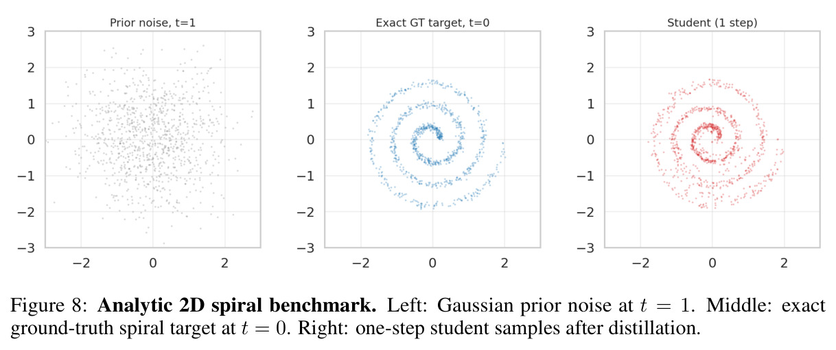
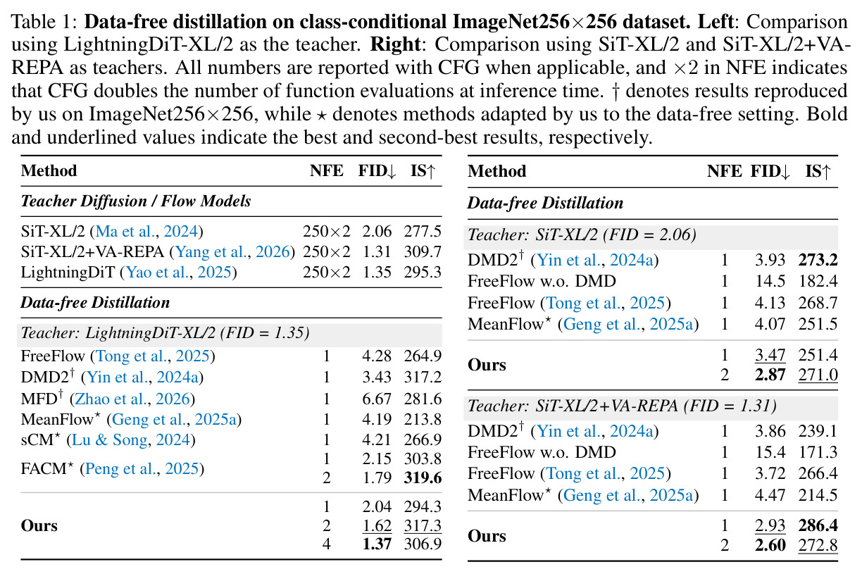
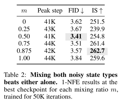
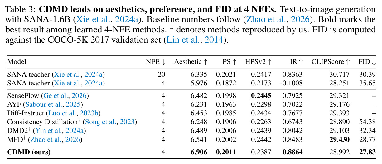
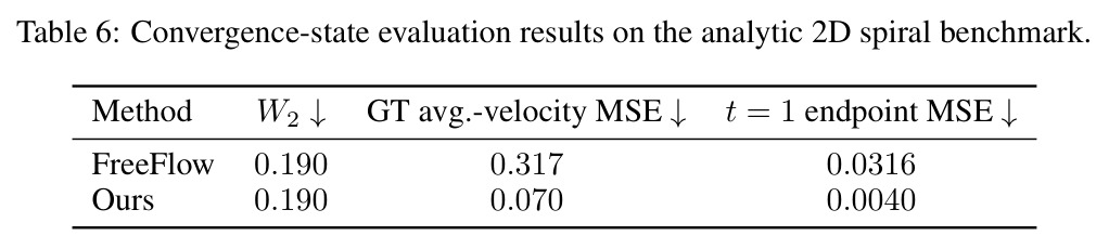
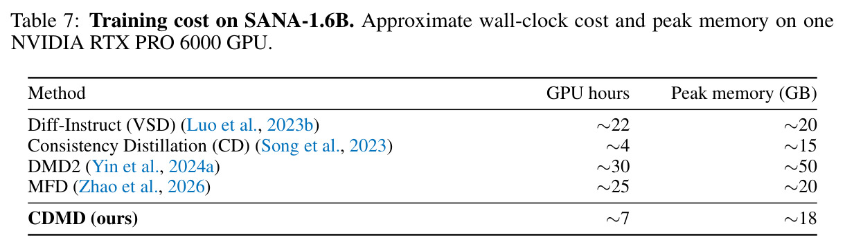
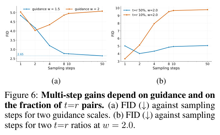
三层实验。(1) 2D螺旋(Table 6):CDMD与FreeFlow的 $\mathcal{W}_2$ 同为0.190,但教师平均速度MSE 0.070 vs 0.317、$t=1$ 端点误差0.0040 vs 0.0316,证明"终点边缘匹配≠输运匹配"。(2) ImageNet 256(Table 1):LightningDiT-XL/2教师(FID 1.35)下CDMD 1/2/4-NFE FID为2.04/1.62/1.37(IS 294.3/317.3/306.9),4步几乎追平教师,同设置FreeFlow 4.28、DMD2 3.43、MFD 6.67、MeanFlow 4.19、sCM 4.21;SiT-XL/2教师下3.47(vs 4.13/3.93/4.07);VA-REPA教师下2.93(vs FreeFlow 3.72);换强教师CDMD改善0.54、FreeFlow仅0.41、DMD2仅0.07、MeanFlow退化。(3) 文生图SANA-1.6B 4-NFE(Table 3):美学6.906、IR 0.8864、FID 27.83为学习类最佳(MFD 28.77、DMD2 32.34),六项全超4-NFE教师,美学/IR/FID超20-NFE教师(30.39),但HPSv2与CLIPScore落后。(4) 成本(Table 7):约7 GPU小时/18GB,vs DMD2约30小时/50GB、MFD约25小时/20GB。(5) 消融:$m=0.5$ 最佳(3.41);$t=r$ 占10%利1-NFE但50步FID约9.8、50%约5.1;深度 $D=8$ 最佳(2.21 vs $D=0$ 的17.60);Euler至8步最优、64步仍贴教师。
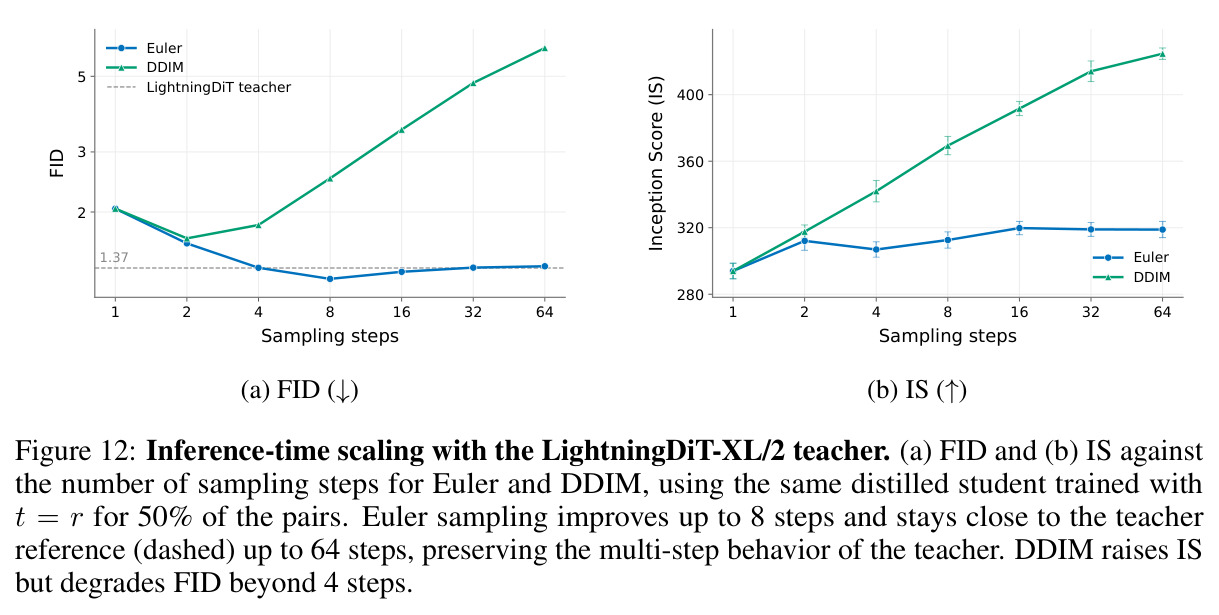
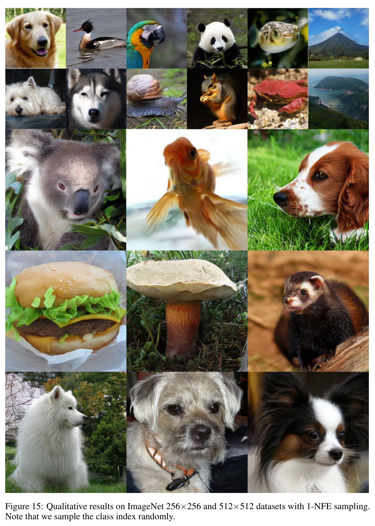
查看结构化数据
| 任务 | 指标 | 本文 | 基线 | 提升 |
|---|---|---|---|---|
| ImageNet 256×256 类条件生成,LightningDiT-XL/2 教师,1步 | FID-50K(越低越好) | 2.04(IS 294.3) | DMD2 3.43 / FreeFlow 4.28 / MeanFlow 4.19 / sCM 4.21(同预算) | 较最佳基线DMD2降低1.39(约40%) |
| ImageNet 256×256,LightningDiT-XL/2 教师,4步 | FID-50K | 1.37(IS 306.9) | 教师扩散模型 1.35(250×2 NFE) | 4步几乎追平500次评估的教师(差距仅0.02) |
| ImageNet 256×256,SiT-XL/2 教师,1步 | FID-50K | 3.47(2-NFE 2.87) | FreeFlow 4.13 / DMD2 3.93 / MeanFlow 4.07 | 较最佳基线降低0.46 |
| ImageNet 256×256,SiT-XL/2+VA-REPA 教师,1步 | FID-50K | 2.93(2-NFE 2.60) | FreeFlow 3.72 / DMD2 3.86 / MeanFlow 4.47 | 较最佳基线降低0.79 |
| 文生图,SANA-1.6B 教师,4步 | FID(对COCO-5K 2017) | 27.83(美学6.906、IR 0.8864) | MFD 28.77 / DMD2 32.34 / Consistency Distillation 54.38 | 较MFD降低0.94,且训练成本约7 vs 25 GPU小时 |
| 2D螺旋合成基准(收敛态) | 教师平均速度 MSE | 0.070(端点MSE 0.0040) | FreeFlow 0.317(端点MSE 0.0316) | 速度场误差降低约78%,端点误差降低约87%(两者W2同为0.190) |
| SANA-1.6B 蒸馏训练成本 | GPU小时 / 峰值显存(单张RTX PRO 6000) | 约7小时 / 18GB | DMD2 约30小时/50GB / MFD 约25小时/20GB / Diff-Instruct 约22小时/20GB | 训练时间降至基线的约1/3~1/4,显存降低2/3以上 |
局限与改进
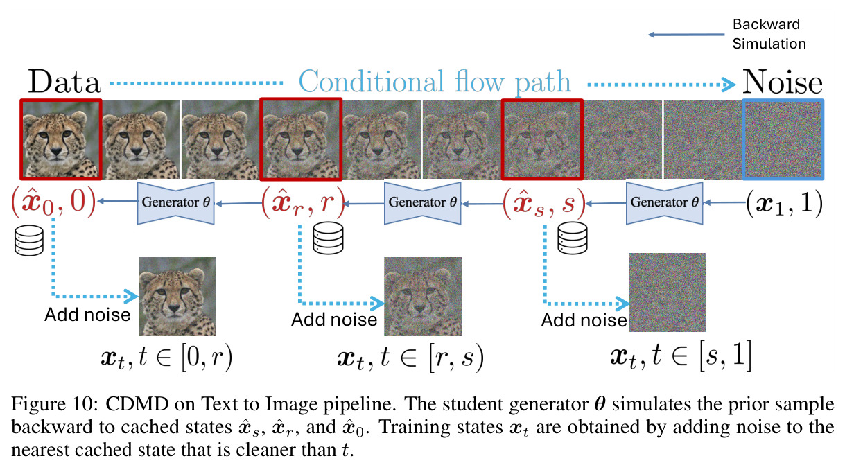
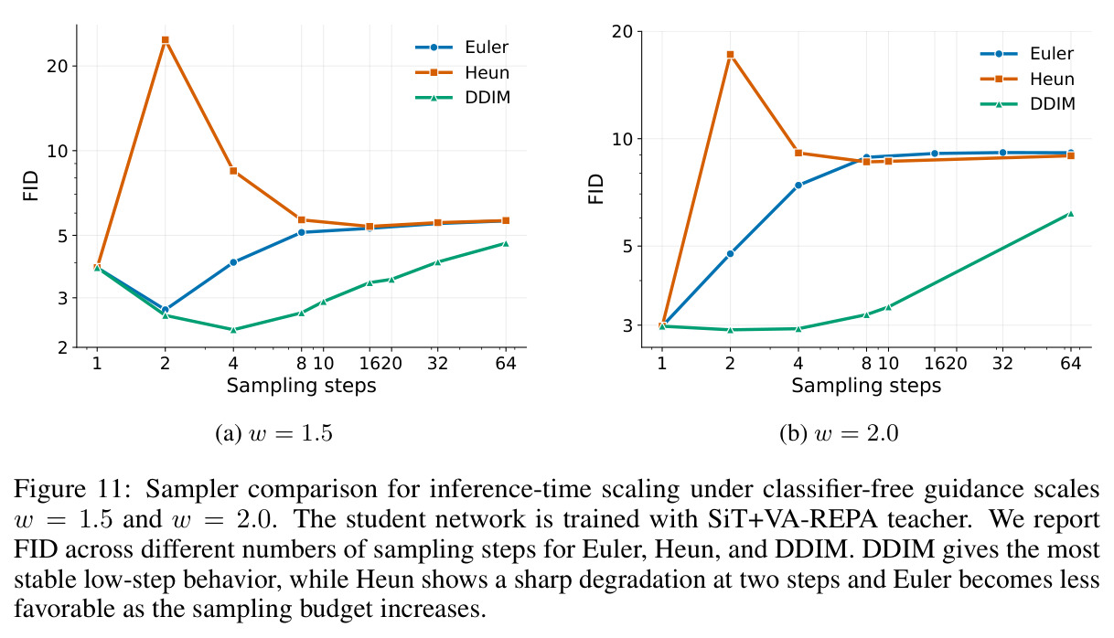
作者承认的局限(附录H):总导数项 $\frac{d}{dt}u(x_t,t,r)=v\,D_xu+\partial_tu$ 缺乏理论约束,其范数在训练中很大且剧烈波动,现有detach处理可能有问题;当教师权重专有时无法用教师权重初始化学生,训练更难更不稳定;$\hat{x}_t$ 的自举方式对任务敏感,可显著影响学习动态与蒸馏效果。我自己的观察:其一,强引导($w=2.0$)下多步采样FID恶化(Fig. 6a),说明学生-教师路径错配会被多步积分放大,推理时必须谨慎选步数与采样器(DDIM最稳、Heun在2步尖锐恶化);其二,文生图上HPSv2与CLIPScore落后(6个基线中分别有4个和5个更高),作者也明说结果"不建立统计优越性";其三,$t=r$ 比例构成1-NFE质量与多步稳定性的权衡,需按部署场景调参;其四,无数据意味着无法用数据纠正教师的缺陷,教师偏差会被蒸馏直接继承;其五,训练依赖定制的Flash-Attention JVP内核,工程复现门槛不低;其六,文生图版要借用TDM式的教师检查点锚定缓存来控漂移,说明纯学生自举在大规模文本条件场景下仍需外部技巧兜底。
独立分析的弱点
独立分析几点弱点并给改进方向。(1) JVP修正项不稳定:作者观测其范数大且训练中剧烈波动,detach等于忽略误差传播。改进:以教师速度场为参考对 $\frac{d}{dt}u_\theta$ 做范数正则,或对该项做EMA/方差缩减。(2) 状态自举偏差:$\hat{x}_t$ 采自 $q_\theta^t$ 而非教师路径,训练早期学生质量差时监督状态偏离教师分布远。改进:设计"教师rollout退火"课程——初期混入少量教师轨迹锚定,随学生提升线性退火到零,兼顾稳定性与数据免费性。(3) 1-NFE与多步质量的权衡源于 $t=r$ 调度:可改为两阶段调度或动态加权,让单一学生同时最优。(4) 强CFG下多步退化:可在目标中加入跨区间自洽项(相邻小区间拼接须与长区间一致),或训练时随机化有效步数模拟推理。(5) 文本对齐指标(HPSv2/CLIPScore)偏弱:可叠加轻量偏好正则或与DPO类后训练组合。(6) 注入深度 $D$ 需网格搜索:可改为可学习门控,让网络自行决定端点信息进入时机。
未来方向
作者明确提出的方向:(1) 提高JVP总导数项的稳定性,例如借助训练良好的参考速度场约束其行为;(2) 在教师权重不可得的场景下设计初始化策略;(3) 把框架推广到数据稀缺问题主导的大规模生成任务(如视频)。基于本文成果可自然延伸:把CDMD用于视频/音频扩散变压器的少步蒸馏,检验JVP在更高维隐空间的表现;将 $t,r$ 调度与端点注入深度自适应化(元学习或可学习调度);收紧理论——去掉contiguity假设、给出非渐近有限样本界,并刻画学生-教师路径错配($M^{JVP}$中的均值偏移项)如何进入误差常数;把"一致性残差⇒分布匹配"的论证推广到随机采样器(SDE)情形;与RLHF/偏好优化结合,在无数据条件下做后训练对齐;以及探索多教师、多分辨率的一致分布匹配与蒸馏中的模型合并。
复现评估
复现条件总体友好。开源:代码与模型在 https://consistentdmd.github.io/ 公开。数据:ImageNet-1K、LAION-Aesthetics 6.5+、COCO-5K均公开。算力:ImageNet蒸馏需683M参数XL学生、100K迭代、batch 1024(lr $3\times10^{-5}$ 或 $1\times10^{-4}$、EMA 0.9995/0.999),属多卡A100级工程量;SANA-1.6B文生图仅约7 GPU小时、峰值18GB,单张RTX PRO 6000即可,门槛很低;2D基准无需大算力,适合先验证实现。两个障碍:一是需仿照sCM实现支持JVP的定制Flash-Attention内核;二是作者自述SiT-XL/2教师设置的"其余配置与评测留空直至训练稳定",说明 $t,r$ 采样分布、引导强度 $w$、EMA速率等仍需试错。综合:小规模验证容易,ImageNet级复现中等难度,需可观但合理的资源。
论文图表
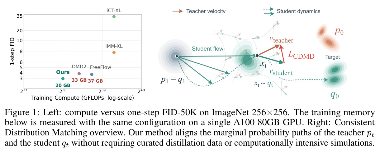
左图在训练算力(GFLOPs,对数轴)与一步FID-50K平面上对比iCT-XL、IMM-XL、DMD2、FreeFlow、LCDMD与本文CDMD,并标注单张A100 80GB上的训练显存(iCT-XL 33GB、IMM-XL 37GB、Ours 20GB);右图示意CDMD对齐教师边缘概率路径 $p_t$ 与学生路径 $q_t$、无需蒸馏数据与高成本模拟的总体框架。
一图点明论文卖点:以显著更低的训练显存取得更好的1步FID,并给出方法全局直觉,是理解全文定位的路线图。