不值得再花一个Token:面向高效深度研究智能体的边际价值估计 Not Worth Another Token: Marginal Value Estimation for Efficient Deep Research Agents
系统比较三阶段边际价值剪枝:早期剪枝最多省73% token且质量基本不变,无单一方法全面占优
前置知识
深度研究智能体与 GPT-Researcher
一类长程 LLM 智能体:把开放式问题分解为子查询,迭代执行检索、把发现累积进上下文、按需派生新子查询,最终综合成带引用的长报告。GPT-Researcher 是其开源实现,默认按宽度 4、深度 3 组织树状搜索,标称搜索树为 $1+4+8+16=29$ 个节点。
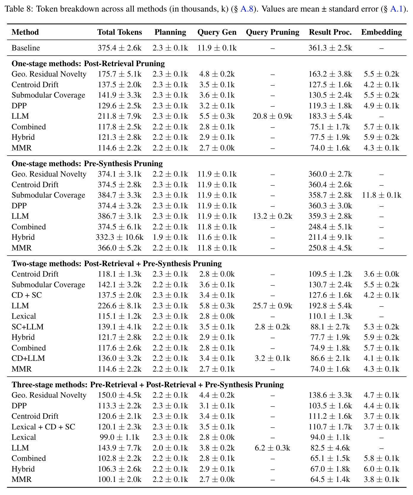
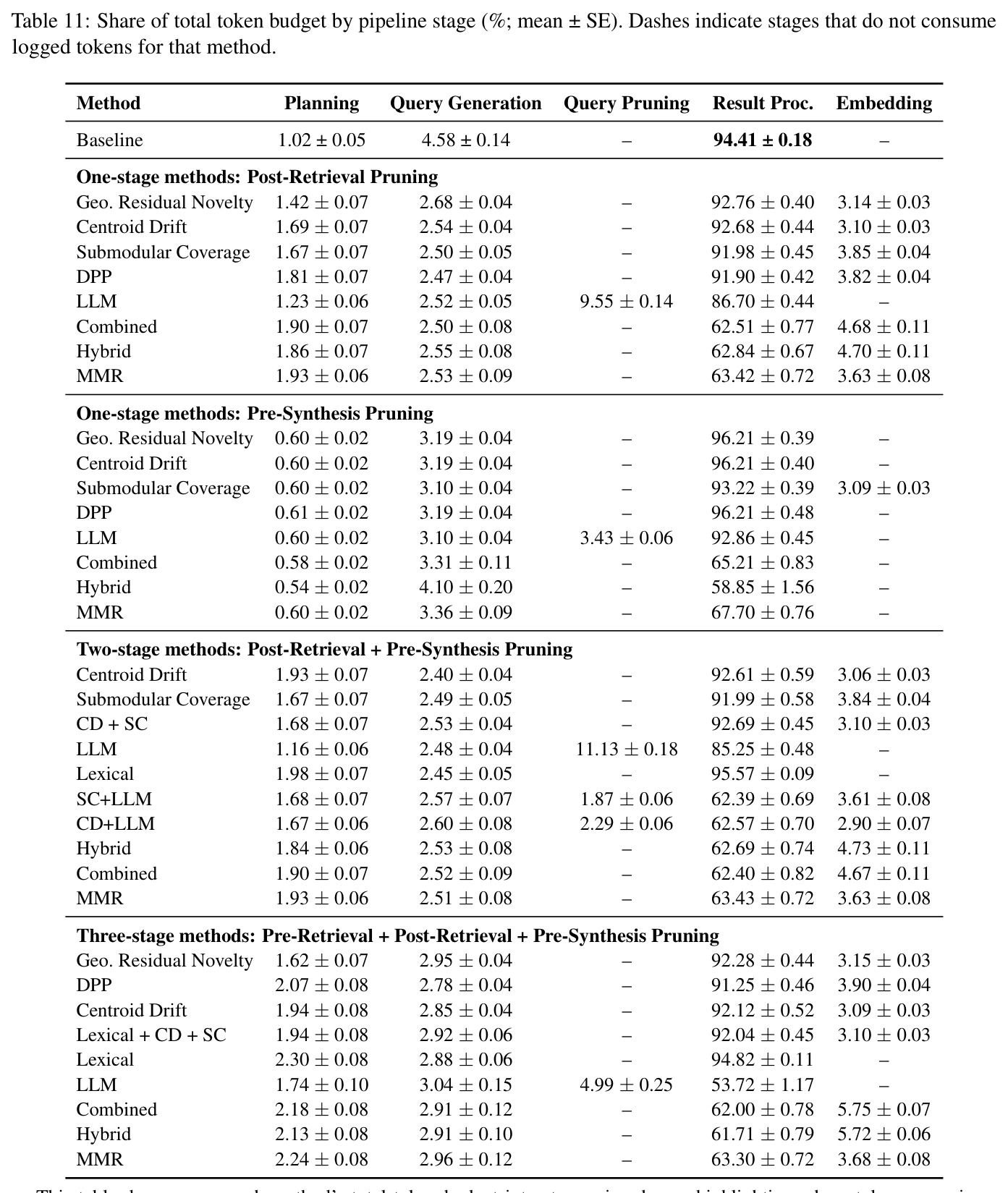
本文所有实验都跑在这条流水线上:三个剪枝点、成本结构(结果处理占 token 的 94.41%)以及基线数字(29.0 节点 / 375.4k token / 3422.6 秒)全部由该框架定义,不懂流水线就无法理解剪枝省在哪。
边际价值估计
借用经济学边际效用思想,估计在已有上下文 $C_t$ 的条件下,新增候选 $x$(子查询或证据块)还能贡献多少新信息。本文统一为打分函数 $V(x \mid C_t, Q)$,低于阶段阈值即丢弃,本质是把不可行的全局子集选择分解为局部贪心决策。
这是全文的方法论主轴:三个剪枝阶段和六类策略(启发式、词汇、LLM、学习式)都是 $V$ 的不同实例化,理解它才能看懂实验设计的因子结构。
最大边际相关性(MMR)
经典检索多样性准则:$V_{\text{MMR}} = \lambda\,\text{sim}(e(x),q) - (1-\lambda)\max_{c\in C}\text{sim}(e(x),e(c))$,第一项奖励与查询相关,第二项惩罚与已选内容冗余,$\lambda$ 控制两者权衡(本文取 0.35)。
MMR 是全场最强压缩器(一阶段省 69.5%、三阶段省 73.3% token),主结论『早期剪枝最有效』主要由它承载,必须理解其相关性-冗余双重目标如何拦截低价值分支。
行列式点过程(DPP)
用半正定核矩阵 $L$ 的行列式度量子集『体积』:元素彼此多样且与查询相关时行列式大。贪心加入使 $V_{\text{DPP}} = \det(L_{C\cup\{x\}})/\det(L_C)$ 最大的候选,冗余项贡献的体积增量趋近于零。
它解释了结果中一个关键分化:DPP 的引用召回最高(一阶段 95.62,超基线 95.54)但压缩不如 MMR——多样性目标倾向保留更宽的证据面,这正是论文『效率与忠实性可分离』论点的例证。
次模函数与贪心覆盖
次模函数具有边际收益递减性质,贪心选择可提供近似保证。本文的次模覆盖 $F(C) = \sum_{i\in C}\max_{j\in P} w(i)\,\text{sim}(e(i),e(j))$ 度量保留集对候选池语义空间的覆盖,并用 token 归一化边际增益 $V_{\text{SC}} = \Delta F(x\mid C)/\text{cost}(x)$ 挑选『覆盖大且便宜』的证据。
SC 是证据保留最好的启发式(三阶段 KPR+KPC 65.79、两阶段引用召回 94.74),与 MMR 构成目标光谱的两端,是理解『无单一方法占优』结论的另一半。
LLM-as-a-Judge
用 LLM 按评分细则给开放文本打分以替代人工评估。本文双重使用:既让 LLM 充当剪枝判官(对每个候选输出 predicted_gain、keep_probability、keep/prune 的 JSON 决策),又让固定裁判按 0-5 对齐细则评报告质量。
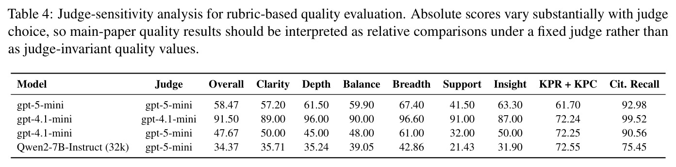
论文最重要的警示来自它:同一批报告在 gpt-4.1-mini 自评下 Overall 91.50,换 gpt-5-mini 裁判只剩 47.67(Table 4)。不理解裁判敏感性就会误读所有质量数字。
稠密嵌入与余弦相似度
把文本映射为向量 $e(x)\in\mathbb{R}^d$,用 $\text{sim}(u,v) = u^\top v/(\|u\|\,\|v\|)$ 度量语义接近程度。MMR/GRN/CD/DPP/SC 全部构建在嵌入空间之上,GRN 还用到向已保留上下文张成子空间的正交投影 $P_C$。
所有启发式剪枝信号都源自嵌入几何(相关性=靠近查询、新颖性=残差/子空间正交分量),不熟悉这套语言就看不懂方法节的公式。
研究动机
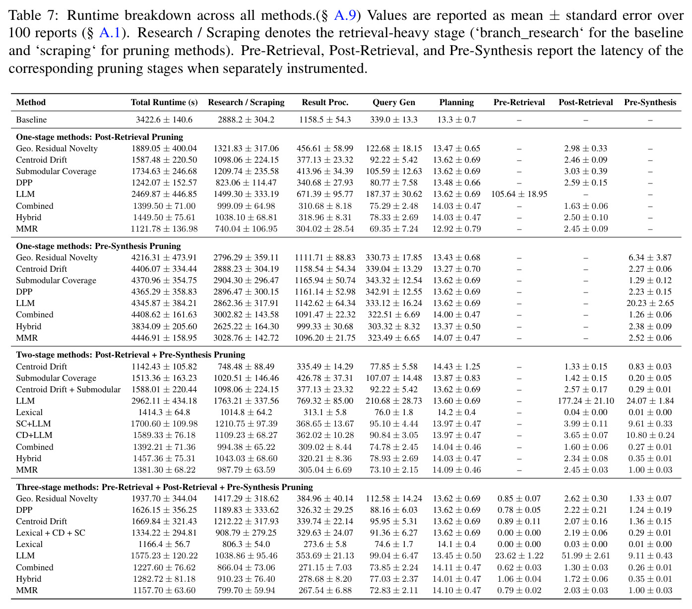
长程研究智能体通过迭代检索、聚合与合成回答开放式复杂问题,但上下文随步骤快速膨胀,而新增证据的边际价值不断递减:早期检索已覆盖核心事实,后期大多带来冗余或弱信息。作者在 GPT-Researcher 风格流水线上的测量显示,未剪枝基线每篇报告平均探索 29.0 个节点、消耗 375.4k token、耗时 3422.6 秒。token 成本高度集中于下游:结果处理阶段占 94.41%,查询生成占 4.58%,规划仅占 1.02%。更关键的是低价值内容存活得太久——框架内置的合成前裁剪只能把累积上下文从 66.10 条压到 44.08 条(条目少 33.3%、token 少 34.06%),而此时检索与处理成本早已付出。这种“太晚”的上下文管理直接推高 token 开销与延迟(每篇报告超过 57 分钟),并向最终报告合成注入噪声。现有工作要么只管探索不管增长(树状深度研究),要么只在最终输入端附近压缩(LLMLingua 等),没有回答“应该在哪一步剪”。
本文的目标是本文的目标是把边际价值估计形式化为深度研究流水线中的阶段感知(stage-aware)剪枝问题,并用受控实验回答三个此前缺乏实证的问题:在哪些阶段剪枝最有效(Pre-Retrieval / Post-Retrieval / Pre-Synthesis)、每个阶段配什么打分规则最好(启发式 / 学习式 / LLM 判官式)、以及报告质量、证据相关性、来源可溯性和成本四个目标在何处发生分化。形式化上,系统在成本预算约束下最大化报告质量:$\max_{C_T} R(C_T, Q)\ \text{s.t.}\ \text{Cost}(C_T) \le B$,等价的拉格朗日形式为 $\max_{C_T} R(C_T,Q) - \eta\,\text{Cost}(C_T)$;由于全局子集优化不可行,作者把它分解为三个局部剪枝点,各自用统一打分函数 $V(x \mid C_t, Q)$ 与阈值 $\tau_{pre}, \tau_{post}, \tau_{syn}$ 做决策,并系统比较一阶段、两阶段、三阶段的组合配置。
与已有工作不同的是,本文的独特切入是把“剪在哪里”提升为与“怎么打分”同等重要的一等设计维度。已有两条线索各缺一半:树状深度研究工作(Tree of Thoughts、ReAct、ParallelResearch)关注如何探索与扩展分支,不控制上下文增长;上下文压缩工作(Lost in the Middle、Selective Context、LongLLMLingua、RECOMP)几乎只在最终模型输入附近压缩,不问干预时机是否比干预手段更重要。作者在完全相同的执行框架下(同一底层搜索策略、同一报告生成配置、跨运行复用缓存的子查询与检索结果)、同一批 100 条查询上,让五族启发式(MMR、GRN、质心漂移、DPP、次模覆盖)、词汇级 TF-IDF 变体、LLM 判官和基于执行轨迹训练的轻量学习控制器,在一/二/三阶段全部组合下同台比较,构成了该问题上的第一个系统性阶段感知实证研究(作者自称 first systematic stage-aware study),并明确承认等预算浅搜索基线缺失这一混淆变量。
核心方法
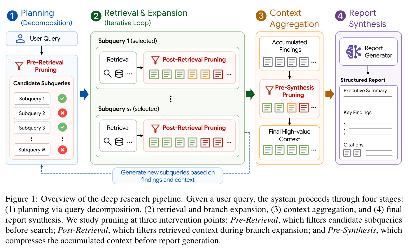
直觉:与其让所有检索结果无差别进入上下文,不如在每个决策点估计候选(子查询或证据块)相对于当前上下文的边际价值,低于阈值就丢弃——“不值得再花一个 token”。技术路线上,系统先把查询 $Q$ 分解为子查询集合 $S$;每步选取 $s_t \in S$ 检索 $C_{s_t}$ 并合并进累积上下文 $C_t$,中间发现还可能派生新子查询动态扩展 $S$。三个剪枝点分别作用于不同成本环节:Pre-Retrieval 在检索发生前过滤低价值子查询,从源头砍掉整棵子树的检索与处理成本;Post-Retrieval 对检索到的条目对照已有上下文打分,丢弃低价值条目以阻止低价值分支的递归扩展;Pre-Synthesis 在报告生成前压缩最终上下文。三者的组合构成一阶段(Post-Retrieval 或 Pre-Synthesis)、两阶段(Post-Retrieval + Pre-Synthesis)与三阶段(全部)配置。所有实验固定在 GPT-Researcher 框架(宽度 4、深度 3,标称树 $1+4+8+16=29$ 个节点)上,Algorithm 1 给出完整流程。
核心创新是把边际价值估计从单一压缩技巧提升为“阶段 × 规则”的因子化设计问题,并证明干预时机往往比打分公式更关键:早期剪枝防止低价值分支“出生”,避免的不仅是最终上下文增长,还有下游检索、结果处理与递归扩展的复合成本;晚期剪枝只能精炼合成提示,无法回收上游开销。第二个关键是统一记号 $V(x \mid C_t, Q)$ 下的异构策略同台比较:相关性-冗余权衡的 MMR $V_{\text{MMR}} = \lambda\,\text{sim}(e(x),q) - (1-\lambda)\max_{c\in C}\text{sim}(e(x),e(c))$;受正交匹配追踪启发的几何残差新颖性 $V_{\text{GRN}} = \|e(x)-P_C(e(x))\|^2$;质心漂移 $V_{\text{CD}} = 1-\text{sim}(\mu_C,\mu_{C\cup\{x\}})$;DPP 增益 $V_{\text{DPP}} = \det(L_{C\cup\{x\}})/\det(L_C)$;token 归一化的次模覆盖 $V_{\text{SC}} = \Delta F/\text{cost}(x)$;以及 LLM 判官与学习控制器。这使“MMR 擅长早期省成本、Hybrid/LLM 擅长晚期提质量”等跨阶段结论成为可能。
方法步骤详情
完整流程(Algorithm 1):(1) 规划器把查询 $Q$ 分解为候选子查询集 $S$,$C_0 \leftarrow \emptyset$;(2) Pre-Retrieval:取出子查询 $s_t$,若 $V(s_t \mid C_{t-1}, Q) < \tau_{pre}$ 则跳过检索;(3) 否则检索得到条目集 $C_{s_t}$,Post-Retrieval 仅保留满足 $V(c \mid C_{t-1}, Q) \ge \tau_{post}$ 的条目并合并进 $C_t$,再据发现派生新子查询加入 $S$;(4) 循环至 $S$ 为空或触发停止条件;(5) Pre-Synthesis:保留 $\tilde{C}_T = \{c \in C_T : V(c \mid C_T, Q) \ge \tau_{syn}\}$;(6) 用 $\tilde{C}_T$ 生成含执行摘要与关键发现的结构化报告。相似度用余弦 $\text{sim}(u,v) = u^\top v/(\|u\|\,\|v\|)$。关键超参:MMR $\lambda=0.35$;GRN $\tau=0.85$;CD $\delta=0.03$;SC 在边际增益/token $<0.05$ 时剪除;Hybrid $(\alpha,\beta,\gamma)=(0.40,0.30,0.30)$。学习控制器用冻结的 BAAI/bge-small-en-v1.5 双塔编码器 + MLP,输出保留概率 $p_{keep}(x)$ 并按阈值剪枝,训练数据为 34 次运行中的 360 个候选分支决策(标签取自次模族运行,按运行切分防轨迹泄漏)。
技术新颖性
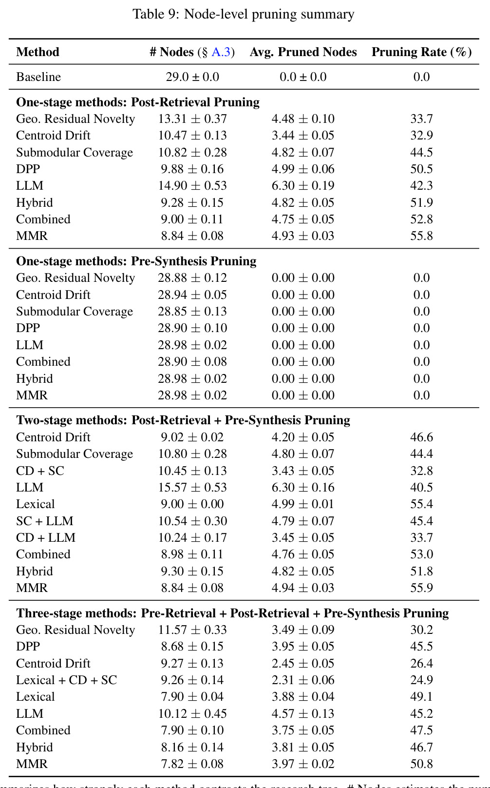
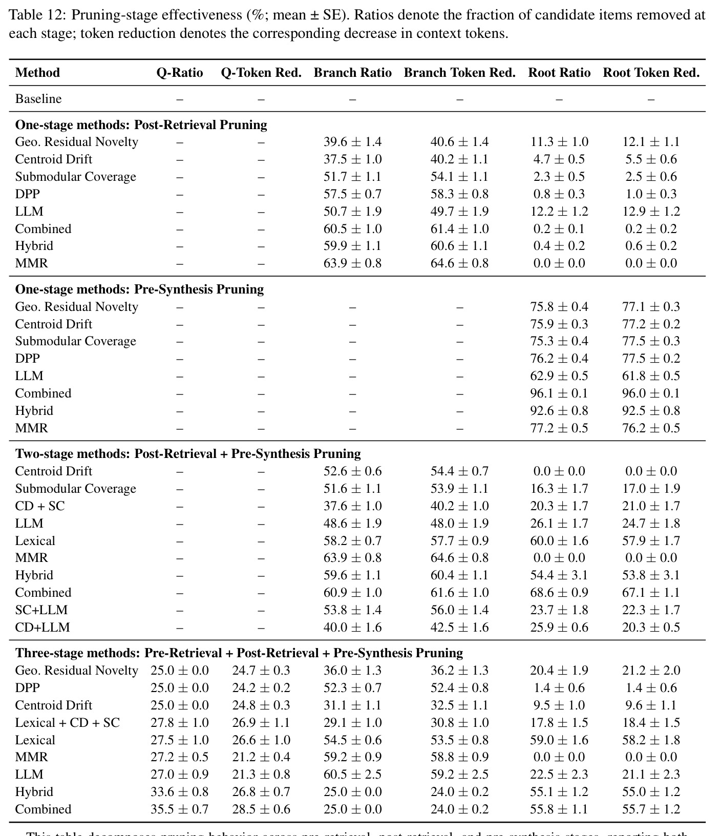
技术新颖性不在单一算法——MMR、DPP、次模覆盖、质心摘要皆为已有技术——而在三点。其一,问题形式化:首次把深度研究智能体的上下文控制表述为覆盖 Pre-Retrieval / Post-Retrieval / Pre-Synthesis 三个干预点及其一/二/三阶段组合的边际价值剪枝问题,并排除了单独 Pre-Retrieval 等部分组合以保证归因清晰。其二,受控归因设计:所有方法共享同一底层搜索策略与报告生成配置,并复用缓存的子查询和检索结果,使观察到的差异可归因于剪枝决策本身;同时诚实声明缺少等预算浅搜索基线,效率增益应理解为“固定搜索策略下的阶段感知剪枝增益”。其三,诊断性度量体系:除总 token 与 runtime 外,还报告节点级剪枝率(如三阶段 MMR 剪掉 50.8% 已探索节点)、阶段级候选删除比例与对应 token 缩减(Table 12),把“成本究竟省在管线哪一层”变成可观测对象,这是以往上下文压缩文献普遍缺失的维度。
实验结果
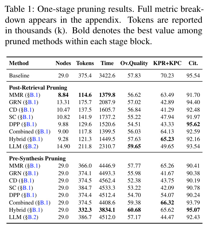
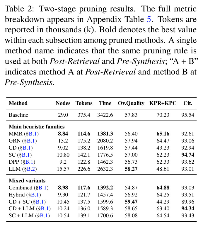
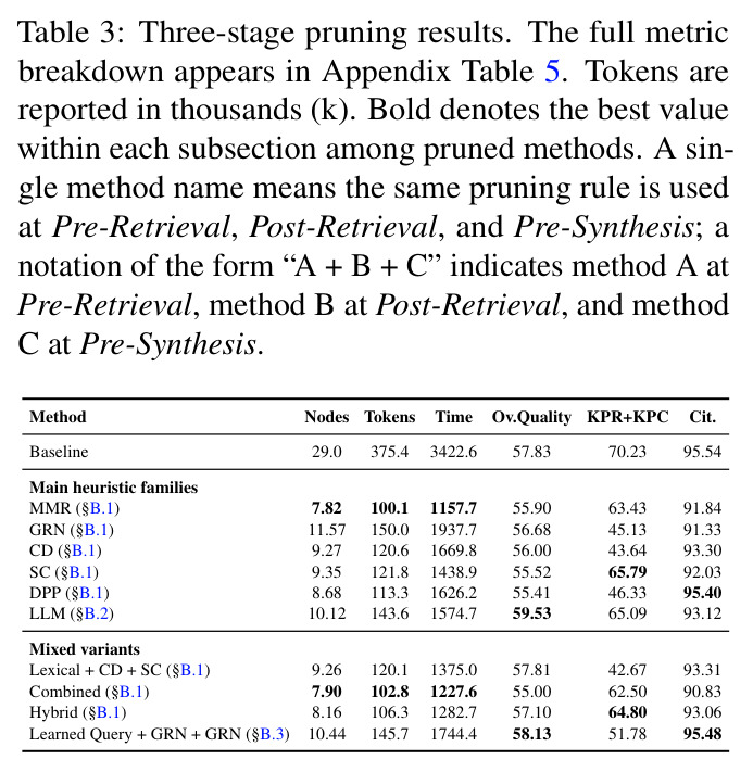
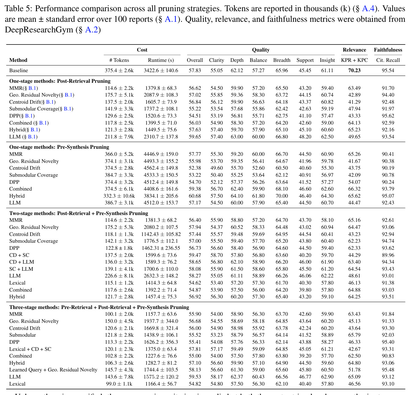
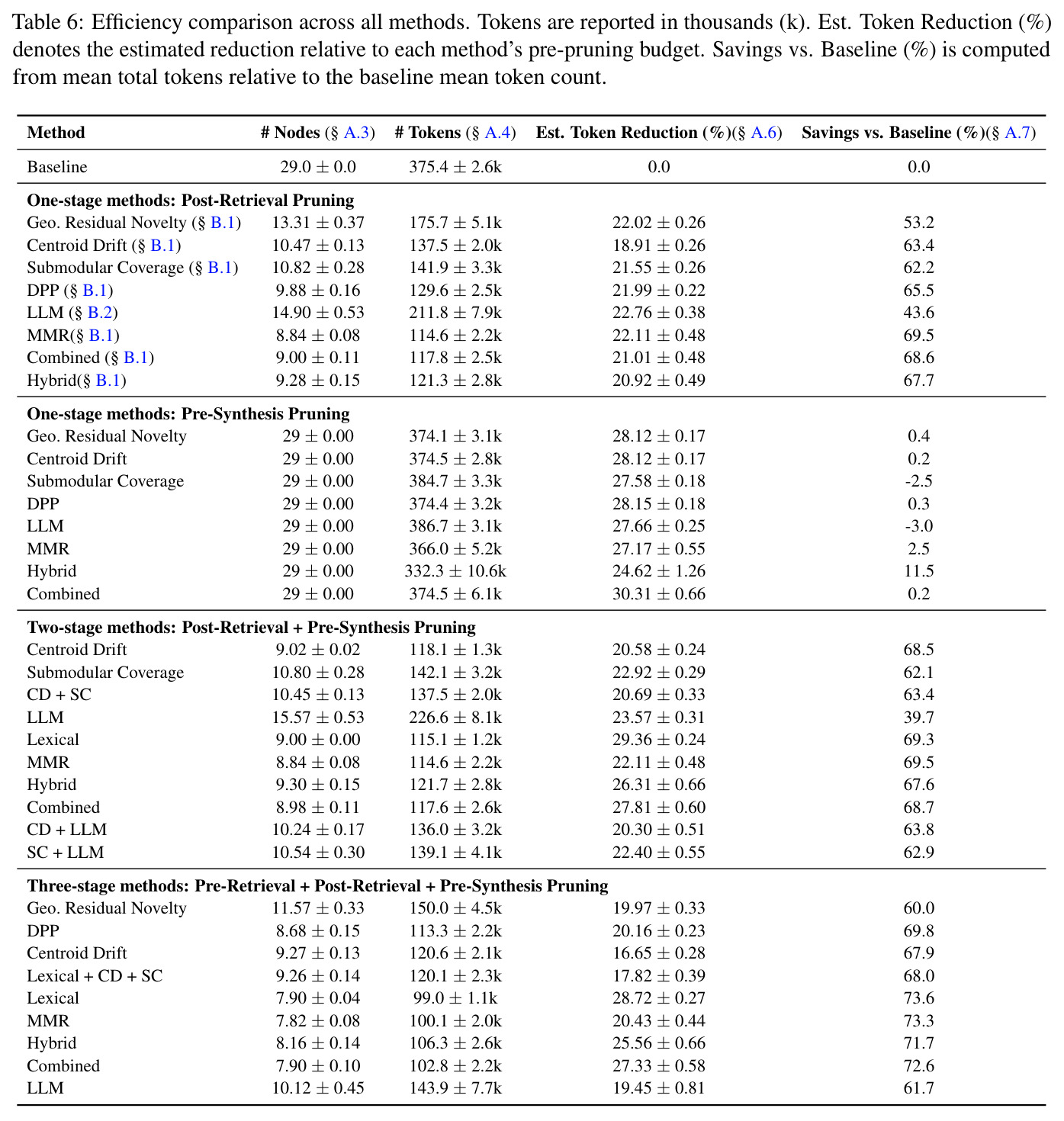
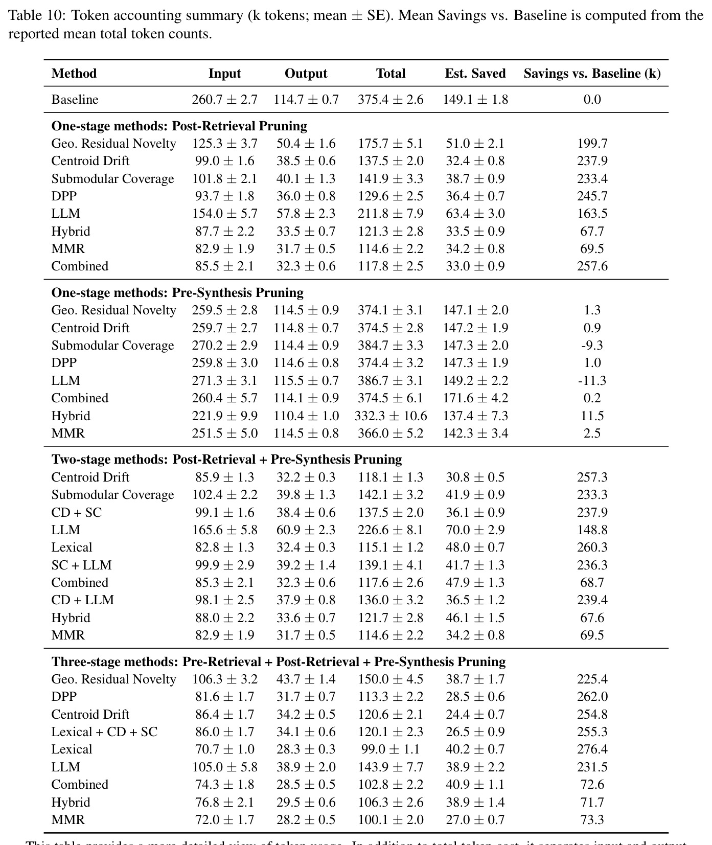
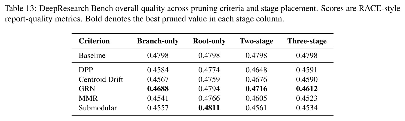
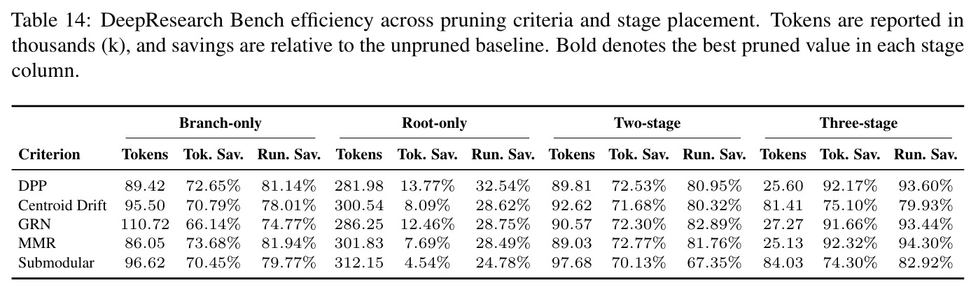
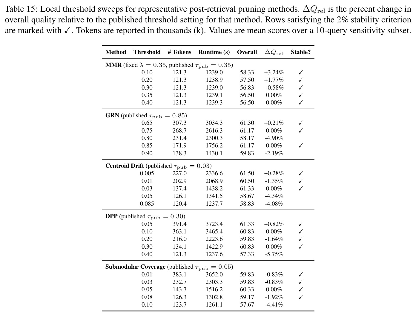
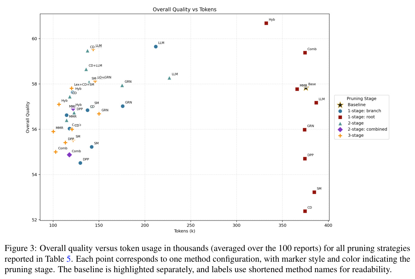
(1) 一阶段:效率最优是 Post-Retrieval MMR——token 375.4k→114.6k(−69.5%),节点 29.0→8.84,runtime −59.7%,质量 56.62(基线的 97.9%);质量最优是 Pre-Synthesis Hybrid(60.68,+2.85),但 token 仅降至 332.3k、runtime 反升至 3834.1s,晚期剪枝无法回收上游成本;无剪枝方法在 KPR+KPC 上超过基线 70.23;引用召回最高是 Post-Retrieval DPP 95.62。(2) 两阶段:最佳折中是 CD+SC——质量 59.47(+1.64),token −63.4%、runtime −53.3%、节点 10.45;MMR 两阶段效率点与一阶段重合(114.6k/8.84),收益在 Post-Retrieval 已拿完;CD+SC 引用召回 89.96 低于 SC 的 94.74,质量与忠实性背离。(3) 三阶段:MMR 压至 100.1k(−73.3%)、节点 7.82、runtime −66.2%,质量 55.90 略降;质量最高是 LLM(59.53),引用召回最强是 Learned Query + GRN + GRN(95.48),KPR+KPC 最高是 SC(65.79)。(4) 跨基准:DeepResearch Bench 上三阶段 MMR 省 92.32% token、94.30% runtime,root-only 仅省 7.69%,效率结论可迁移而质量排名不稳。(5) 裁判敏感性:同一批报告换裁判从 91.50 跌至 47.67。(6) 阈值扫描:五个代表性方法的发布阈值均在 2% 稳定区间内。
查看结构化数据
| 任务 | 指标 | 本文 | 基线 | 提升 |
|---|---|---|---|---|
| 端到端成本(一阶段 Post-Retrieval MMR) | 总 token / runtime | 114.6k / 1379.8s | 375.4k / 3422.6s(无剪枝 GPT-Researcher) | token −69.5%,runtime −59.7% |
| 端到端成本(三阶段 MMR,最大压缩) | 总 token / runtime / 节点 | 100.1k / 1157.7s / 7.82 | 375.4k / 3422.6s / 29.0 | token −73.3%,runtime −66.2%,节点 −73.0% |
| 报告质量(一阶段 Pre-Synthesis Hybrid) | Overall Quality(固定 LLM 裁判) | 60.68 | 57.83 | +2.85(但 token 仅省 11.5%) |
| 质量-效率折中(两阶段 CD + SC) | Overall Quality + token | 59.47,137.5k token | 57.83,375.4k token | 质量 +1.64,token −63.4%,节点 29.0→10.45 |
| 证据相关性保留 | KPR+KPC | 65.79(三阶段 SC,剪枝方法最高) | 70.23 | −4.44;所有剪枝方法均未超过基线 |
| 来源可溯性 | Citation Recall | 95.48(三阶段 Learned Query + GRN + GRN);一阶段 Post-Retrieval DPP 95.62 | 95.54 | 基本持平(−0.06 ~ +0.08) |
| 跨基准效率验证(DeepResearch Bench,三阶段 MMR) | token / runtime 节省 | 92.32% / 94.30% | 无剪枝基线(0.4798 RACE 质量) | 效率结论跨基准成立;root-only 仅省 7.69% token |
| 裁判稳健性 | Overall(同一报告,换裁判) | gpt-4.1-mini 报告被 gpt-5-mini 评 47.67 | gpt-4.1-mini 自评 91.50 | 绝对分不可跨裁判比较,仅相对比较有效 |
局限与改进
作者承认的局限:实验绑定单一流水线(GPT-Researcher)与基准(DeepResearchGym 的 100 条查询子集),结论是“该设置下的比较研究”而非普适定律;缺少等预算浅搜索基线,效率增益无法与“单纯缩小搜索预算”区分;质量分数强依赖裁判模型,绝对值跨裁判大幅漂移(91.50 vs 47.67),只有固定裁判下的相对比较可信;阈值与超参选择任务相关,细粒度方法排序可能随阈值移动;自动指标(质量、KPR+KPC、引用召回)不能覆盖事实正确性、证据完整性与对终端用户的有用性。我的补充观察:100 条查询下 ±2 分量级的质量差异多在标准误噪声范围内,统计功效有限;KPR+KPC 系统性下降(如 Post-Retrieval GRN 一阶段掉至 42.89,比基线低 27.3 分)意味着剪枝持续丢失证据覆盖,但正文对此着墨不多;学习控制器仅有 360 个训练决策点且标签来自单一策略族(submodular 运行),“学习式不敌启发式”的结论可能是数据规模伪影;此外未报告检索 API 调用次数的货币成本,也未测试更换嵌入模型对剪枝信号质量的敏感性。
独立分析的弱点
(1) 证据保留与裁判分脱钩——几乎所有剪枝配置的 KPR+KPC 低于基线(Post-Retrieval GRN 一阶段 42.89 vs 70.23),报告流畅却悄悄丢掉反例、少数观点与关键警告,高风险场景危险。改进:把覆盖率约束并入剪枝目标(如带覆盖下界的次模选择),或为被剪证据维护“影子索引”供引用审计回捞。(2) 无等预算对照——效率增益可能主要来自“搜得少”而非“剪得准”。改进:加入宽度/深度减半的静态浅搜索基线,验证边际价值标准在同预算下仍占优。(3) 绝对阈值跨域脆弱——MMR λ=0.35、GRN τ=0.85 等均在 100 条查询上调出,换领域需重标定。改进:改用分位数自适应阈值(每步保留 top-k%)或在线校准。(4) LLM 判官自身开销大——其一阶段 Post-Retrieval 剪枝耗 20.8k token(占总预算 9.55%)、延迟 105.6s,token 节省率 43.6% 全场最低。改进:小模型蒸馏判官决策或批量裁决。(5) 单一嵌入模型依赖——所有启发式共享一个嵌入空间。改进:网格化嵌入模型与维度,报告方法排序稳定性。
未来方向
作者提出的方向:增加等预算浅搜索基线作为对照;在多个独立裁判下检验方法级排序的稳定性;把学习式剪枝从 360 决策点的概念验证扩展为成熟方案;构造覆盖有用性与可靠性的评估指标。基于本文成果可延伸:(1) 自适应阶段路由——按查询复杂度与风险等级动态选择一/二/三阶段配置,论文的跨阶段结论已构成天然决策表(极致压缩用三阶段 MMR,质量优先用两阶段 CD+SC 或一阶段 Pre-Synthesis Hybrid);(2) 用 KPR+KPC 类覆盖率信号闭环在线调阈值,形成“检索-剪枝-评估”自监督回路,缓解证据覆盖静默流失;(3) 学习控制器的规模化——用大量廉价的次模标签预训练再小样本微调,检验“启发式够用”的结论在 10 倍数据下是否仍成立;(4) 与树状自适应资源分配(如 ParallelResearch)正交结合:边际价值剪枝决定哪些分支不该出生,资源分配决定存活分支获得多少预算;(5) 面向表格、图表等多模态证据定义边际价值与覆盖度量;(6) 把 token 节省换算为货币成本与碳排放节省,定量落实伦理声明中的环境收益主张。
复现评估
所有组件开源可得:GPT-Researcher 框架、DeepResearchGym 评估沙盒(协议基于 Researchy Questions 的 1000 条查询,本文取固定 100 条)、公开嵌入模型 BAAI/bge-small-en-v1.5;Algorithm 1 伪代码、全部超参(MMR λ=0.35、GRN τ=0.85、CD δ=0.03、SC 阈值 0.05、Hybrid 0.40/0.30/0.30 等)、完整提示词(Figure 2)与带标准误的完整结果表(Tables 5-15)齐备,信息完备性属实证论文上乘。主要门槛是预算而非技术:基线每篇报告 3422.6 秒、375.4k token,十几种配置 × 三种阶段组合 × 100 查询意味着单轮完整评估达数千万 token 量级(约数千美元 API 费用),LLM 裁判还需额外调用 gpt-5-mini / gpt-4.1-mini。论文未明确承诺公开代码,且剪枝执行依赖跨运行复用缓存子查询与检索结果的框架,复现者需自行重建以保证可比性;网页检索非确定性会使绝对数值漂移,但 69-73% 的节省量级应稳健。总体:中等偏易,建议先在 10-20 条查询上复现关键对照(基线 vs Post-Retrieval MMR vs 三阶段 MMR)。
论文图表
展示两段实际提示词:(a) LLM 查询剪枝指令——输入根查询、当前框架查询、父研究目标与候选查询列表,要求对每个候选输出 predicted_gain、keep_probability、keep/prune 决策及理由,且只返回 JSON;(b) LLM-as-a-judge 评估指令——对候选问答与标准答案的语义对齐度按 0-5 打分(5 为完全对齐、0 为无关或矛盾)。
LLM 判官式剪枝与 LLM 裁判评估的具体实现完全由这两段提示词定义,是复现实验和评估其设计选择(保守剪枝原则、仅输出整数等)的直接依据。