← 返回 2026-05-05

基于轨道空间粒子流匹配的生成建模 Generative Modeling with Orbit-Space Particle Flow Matching

Sinan Wang, Jinjin He, Shenyifan Lu, Ruicheng Wang, Greg Turk, Bo Zhu 📅 2026-05-04 👍 9 2026-07-13 08:36
几何深度学习 流匹配 生成模型 粒子系统 计算机图形学

OGPP:用轨道规范化+索引嵌入+几何路径统一粒子生成的对称性与属性编码

前置知识

Flow Matching (流匹配)

流匹配是连续时间生成建模框架,通过学习速度场 $u_\theta^t(X_t,t)$ 沿 ODE 积分把噪声分布 $p_{\text{init}}$ 输运到数据分布 $p_{\text{data}}$。训练用条件流匹配损失让网络回归参考速度场,无需模拟即可学向量场。

OGPP 是流匹配框架的粒子系统特化版本,必须先理解标准流匹配如何用 ODE 输运分布,才能理解 OGPP 引入的轨道空间和几何概率路径对流匹配的核心修改。

Permutation Symmetry (置换对称性)

粒子系统的根本性质:$N$ 个粒子索引任意调换都不改变底层物理配置。从群论角度,所有置换相关配置构成同一轨道 $\text{Orb}(x) = \{\rho(g)x : g \in S_N\}$,但把粒子拉成向量表示时置换会任意改变向量化结果。

OGPP 的核心动机之一就是处理置换对称性。图像像素在固定网格坐标上的统计一致性无法迁移到粒子系统,所以 OGPP 提出对 $X_1$ 做轨道空间规范化,把粒子索引变成'可学习的角色分配'。

Orbit-Space Canonicalization (轨道空间规范化)

规范化映射 $C: \mathbb{R}^d \to \mathbb{R}^d$ 从每个等价轨道选出一个代表元,要求 (1) $G$-不变性;(2) $C(x) \in \text{Orb}(x)$。粒子系统中可用 Hilbert 曲线、Z-order 等空间填充曲线实现。

OGPP 三大组件之首。论文通过总协方差分解证明规范化 $X_1$ 后条件协方差中'角色模糊项'消失,使速度回归任务本质上更容易学。

Hermite Curve (Hermite 曲线)

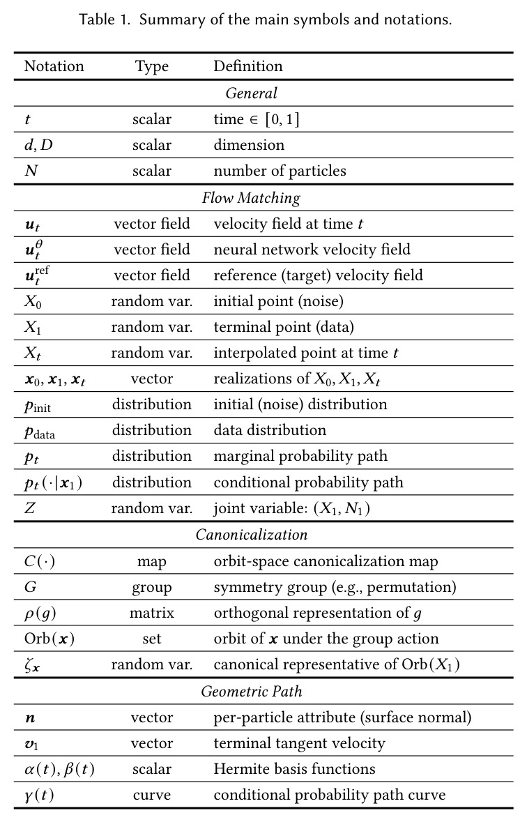
Hermite 曲线是满足端点位置和切向约束的多项式插值。二次 Hermite 用 $\alpha(t)=2t-t^2$、$\beta(t)=t^2-t$ 自动满足 $\gamma(0)=x_0$、$\gamma(1)=x_1$、$\dot{\gamma}(1)=v_1$。

OGPP 用二次 Hermite 曲线构造几何概率路径,把表面法向 $n_1$ 编码进终端切向 $v_1 \propto n_1$,使学习到的流在 $t=1$ 时同时给出粒子位置和法向,无需额外网络输出。

Energy-Driven Particle Systems (能量驱动粒子系统)

粒子配置由物理/几何能量泛函的极小化定义。蓝噪声寻求低频抑制各向同性点集;最小曲面在给定边界下最小化面积;DLA 模拟布朗运动附着形成分形;Thomson 问题求 $N$ 电荷库仑排斥极小解。

OGPP 的第三个贡献是提出针对能量驱动粒子系统的内禀度量(功率谱、面积分数误差、分形维数、库仑残余力),弥补传统生成模型只看 1-NNA 等分布匹配指标的不足。

研究动机

现代主流生成模型 (diffusion、flow matching) 都建立在规则欧几里得网格上,天然适合图像和视频,因为像素在固定坐标上的统计性质在样本间稳定。然而粒子系统 (点云、Lagrangian 流体、agent 仿真) 在物理空间中定义,本质上有两个根本差异:第一,置换对称性——$N$ 个粒子索引任意调换不改变底层配置,但会把高维向量表示随意映射到不同位置,导致每个固定索引 $i$ 对应的回归目标在样本间剧烈分散,速度场被迫对'互不相容的目标'做平均;第二,物理意义——在流匹配 ODE 中,$t=1$ 时的终端速度在像素生成里没有几何含义,但在粒子系统中可以天然编码局部几何信息 (如表面法向),而标准线性插值路径完全浪费了这个自由度。现有粒子生成器如 Equivariant Flow Matching 用 OT 耦合缓解置换模糊,但训练复杂度高达 $O(B^2N^3)$,扩展性差;NSOT 改进可扩展性但仍依赖匿名粒子表示,单个索引必须聚合多种对称诱导的角色,目标方差大、轨迹严重弯曲。

本文的目标是提出一个粒子原生的生成框架 (OGPP),同时实现三个目标:(1) 把每个粒子的条件协方差降到下界,让每个索引对应一个稳定、局部的空间区域,从而降低 Bayes-optimal 速度场的不可约 MSE;(2) 通过轨道连续的规范化映射使 Bayes-optimal 速度场本身是局部 Lipschitz 的,鼓励直 (straight) 流,从而用极少的 ODE 步数 (single-step 或 few-step) 完成高质量生成;(3) 把终端速度这个原本'未使用'的自由度变成每粒子几何属性 (如表面法向) 的载体,让一个流同时生成位置和属性,无需额外网络分支。具体可量化目标:在最小曲面生成上单步即达到面积误差 < 0.005,比基线 (0.7) 提升两个数量级;在 ShapeNet 飞机上用 26M 参数 + 200 步达到 EMD 58.77,与 DiT-3D XL (675M, 1000 步) 的 58.67 相当但少 26 倍参数和 5 倍步数。

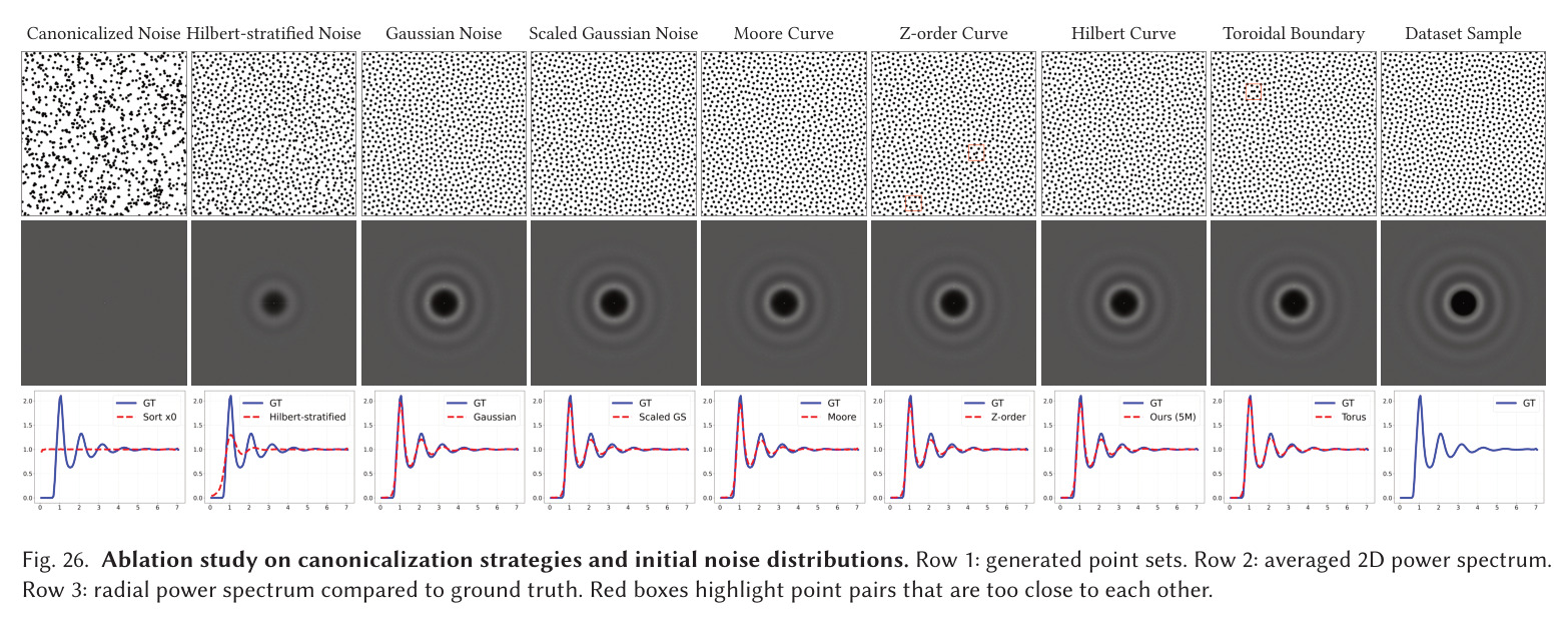
与已有工作不同的是,现有工作要么只在架构层面做对称性 (置换等变网络),要么用 OT 耦合做软对齐,但都回避了轨道空间的离散几何。OGPP 的独特切入角度是把规范化 (canonicalization) 和路径设计 (path design) 联合起来:观察到对 $X_1$ 单边规范化能在条件协方差和 Lipschitz 比之间取到最优折衷,进一步设计几何概率路径利用终端切向编码几何属性,最后用基于 Hilbert 曲线排序的实用算法把这些理论性质落地,形成端到端的 Lagrangian 视角粒子生成框架。与 NSOT 等基于 OT 的方法相比,OGPP 避免了昂贵的 $O(B^2N^3)$ 耦合;与 EqFM 等严格等变方法相比,OGPP 通过规范化把'刚性对称'转为'学习到的稳定索引',允许更灵活的容量分配。

核心方法

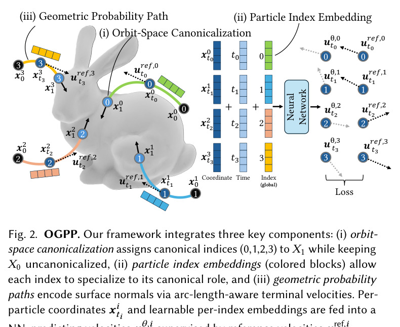
OGPP 把'粒子生成'重新诠释为'粒子在物理空间中沿学习到的 ODE 流演化'的 Lagrangian 过程,不像图像生成那样把粒子位置作为固定网格上的值来填。具体方法可以这样类比:想象 $N$ 个有名字的特工 (粒子),他们要从随机站位 (噪声 $X_0$) 出发走到目标位置 $X_1$ 并站好面向正确的方向 (法向)。传统流匹配把所有特工匿名编号,导致'特工 0 号'今天被指派去左边、明天被指派去右边,他必须同时学两个任务;OGPP 给每个特工发一个固定身份徽章 (particle index embedding),再给所有配置按 Hilbert 空间填充曲线排个序,让'特工 0 号'永远站在最左下角 (canonicalization),这样他只需要学好一个稳定任务。同时,传统流匹配用直线插值轨迹,OGPP 改用二次 Hermite 曲线,额外允许轨迹在终点以一定切向 (与法向对齐) 着陆,把特工到达位置时的'朝向'这个原本被忽略的信息利用起来。在训练时只用 3D 坐标做 ODE 积分,推理时把 $t=1$ 时的速度方向取出,归一化就是表面法向。

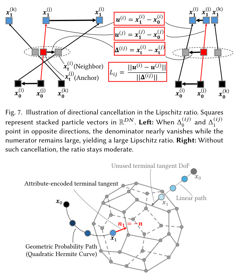
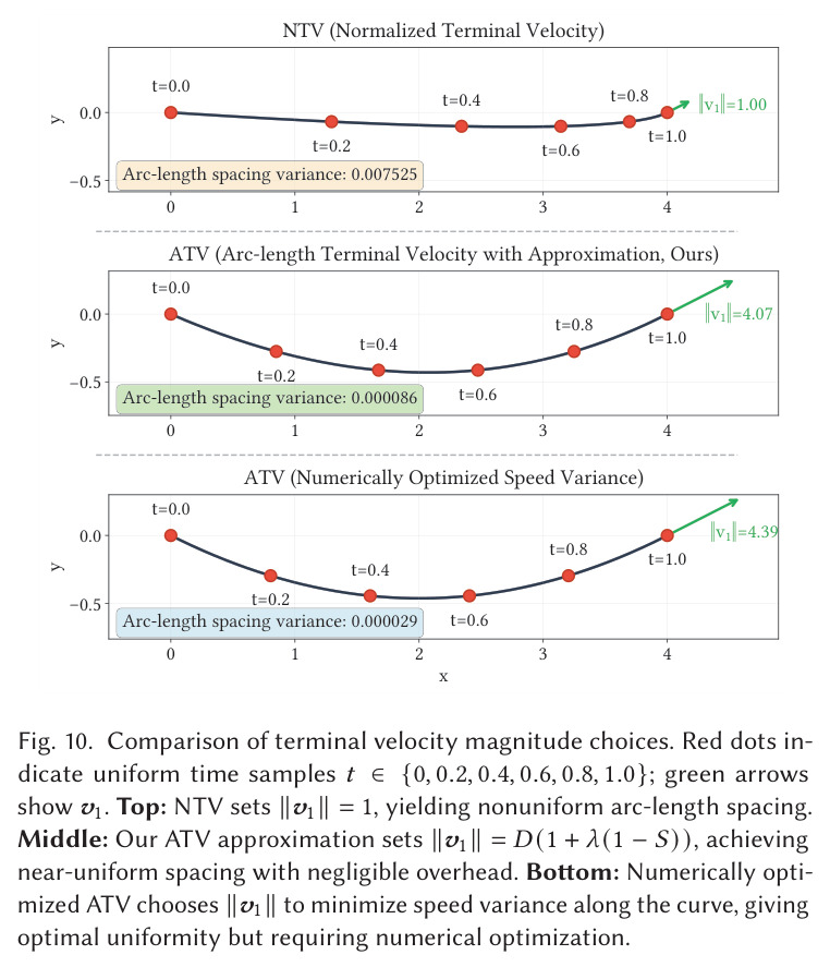
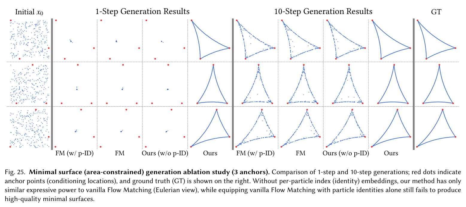
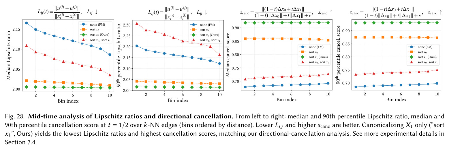
OGPP 与已有粒子生成器最本质的区别在于三点:(1) 它把'规范化'从数据预处理变成概率路径端点的设计选择——只规范化 $X_1$、保留 $X_0$ 的随机性,从协方差分解上消除角色模糊项而不会引发方向对消 (directional cancellation),从而在条件协方差与 Lipschitz 比率之间取得最优折衷;(2) 它把'终端速度'从无意义的自由度变成每粒子几何属性的载体——通过二次 Hermite 曲线 $\gamma(t) = x_0 + \alpha(t)(x_1 - x_0) + \beta(t)v_1$ 把法向嵌入 $v_1 \propto n_1$,并用 ATV 缩放 $L_{\text{arc}} = D(1+\lambda(1-S))$ 让轨迹沿弧长近似匀速;(3) 它用 Lagrangian 视角把所有这些组件协同起来:identity embedding 让每个索引学会一个稳定的角色,canonicalization 让角色之间不冲突,几何路径让流在终点自然编码属性。三者缺一不可——单独加 index embedding (Figure 25) 或单独做规范化都不能复现完整 OGPP 的性能,这是和 Equivariant Flow Matching 等架构层面等变方法最大的不同。

方法步骤详情

OGPP 的完整训练流程如下 (Algorithm 1):(1) 从数据集 $\mathcal{D} = \{(x_1^{(j)}, n_1^{(j)})\}_{j=1}^M$ 采样 $(x_1^{(i)}, n_1^{(i)})$;(2) 采样噪声 $x_0^{(i)} \sim \text{Uniform}([-1,1]^N)$;(3) 对 $(x_1, n_1)$ 做联合规范化:6D Hilbert 曲线在 $(x_1, n_1)$ 联合空间中排序,最小曲面任务则用逆时针多边形排序;(4) 对每个粒子 $k$ 并行计算弦长 $D = \|x_1 - x_0\|$、弦方向 $\hat{d}$、单位法向 $\hat{n}_1$、对齐度 $S = \hat{d} \cdot \hat{n}_1$、ATV 长度 $L_{\text{arc}} = D(1+\lambda(1-S))$ 和终端速度 $v_1 = L_{\text{arc}} \hat{n}_1$;(5) 用 $\alpha(t)=2t-t^2$、$\beta(t)=t^2-t$ 构造 Hermite 曲线 $\gamma(t)$;(6) 采样 $t \sim \text{Uniform}([0,1])$,沿曲线计算 $x_t^{(i,k)} = \gamma(t)$ 和参考速度 $u_t^{\text{ref}} = \frac{2(x_1 - x_t)}{1-t} - v_1$;(7) 神经网络 (Transformer encoder) 输入每粒子 embedding $\boldsymbol{h}_i^{(0)} = W_{\text{in}} x_i^t + e_i + \phi_t(t)$(含粒子索引嵌入 $e_i$ 和时间嵌入 $\phi_t$),输出预测速度 $u_{\theta,i}^t$;(8) 计算 MSE 损失 $\mathcal{L} = \frac{1}{N}\sum_k \|u_{\theta,k}^t(x_t) - v_t^{(k)}\|^2$ 并反向传播。推理 (Algorithm 2):(1) 采样 $x_0 \sim \text{Uniform}([-1,1]^N)$;(2) 用 ODE 求解器 (RK 或 Euler) 从 $t=0$ 积分到 $t=1$,步长 $\Delta t = 1/K$;(3) 在 $t=1$ 取出终端速度 $v_i^1 = u_{\theta,i}^1(x_1)$,归一化 $\hat{n}_i = v_i^1 / \|v_i^1\|$ 即得每粒子法向。网络是 plain Transformer encoder,可选地插入 cross-attention 处理条件任务 (如最小曲面的锚点)。

技术新颖性

OGPP 的新颖性体现在三个层面。第一,理论层:第一次给出粒子系统条件协方差的总方差分解 (Equation 7),明确分离'内在变差'与'角色模糊项',并证明规范化使后者为零;同时通过 Lipschitz 比率分析证明'只规范化 $X_1$、不规范化 $X_0$'在方向对消意义下是最优的——把 $X_0$ 也规范化会让 $\Delta_0^{(ij)}$ 和 $\Delta_1^{(ij)}$ 同尺度,引发分母近零、数值不稳定。第二,路径设计层:第一次把二次 Hermite 曲线的终端切向作为表面法向的载体,并提出 ATV 缩放公式,使 Hermite 路径同时满足几何属性编码和弧长匀速,避免手工调度。第三,评估层:第一次系统提出能量驱动粒子系统的内禀度量 (蓝噪声功率谱 Pearson 相关性与 $L_2$ 误差、最小曲面面积分数误差与角度平滑度、DLA 分形维数、多层 Thomson 残余库仑力),把生成模型评估从纯分布匹配推进到物理保真度评估。和 gVP (Chang et al. 2024) 等仅在 latent 空间编码法向的工作相比,OGPP 在 3D 物理空间中以无额外成本的方式完成法向生成。
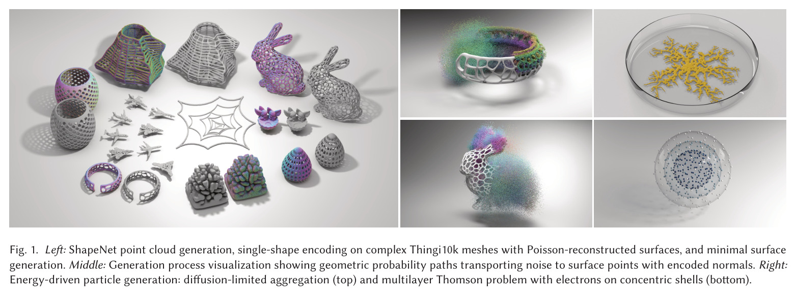
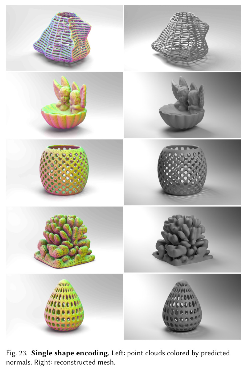
Left: ShapeNet point cloud generation, single-shape encoding on complex Thingi10k meshes with Poisson-reconstructed surfaces, and minimal surface generation. Middle: Generation process visualization showing geometric probability paths transporting noise to surface points with encoded normals. Right: Energy-driven particle generation: diffusion-limited aggregation (top) and multilayer Thomson problem with electrons on concentric shells (bottom).
Fig. 1: Left: ShapeNet point cloud generation, single-shape encoding on complex Thingi10k meshes with Poisson-reconstructed surfaces, and minimal surface generation. Middle: Generation process visualization showing geometric probability paths transporting noise to surface points with encoded normals. Right: Energy-driven particle generation: diffusion-limited aggregation (top) and multilayer Thomson problem with electrons on concentric shells (bottom).
OGPP. Our framework integrates three key components: (i) orbit-space canonicalization assigns canonical indices (0,1,2,3) to X1 while keeping X0 uncanonicalized, (ii) particle index embeddings (colored blocks) allow each index to specialize to its canonical role, and (iii) geometric probability paths encode surface normals via arc-length-aware terminal velocities. Per-particle coordinates x_t^i and learnable per-index embeddings are fed into a NN, predicting velocities u_theta,i^t supervised by reference velocities u_ref,i^t.
Fig. 2: OGPP. Our framework integrates three key components: (i) orbit-space canonicalization assigns canonical indices (0,1,2,3) to X1 while keeping X0 uncanonicalized, (ii) particle index embeddings (colored blocks) allow each index to specialize to its canonical role, and (iii) geometric probability paths encode surface normals via arc-length-aware terminal velocities. Per-particle coordinates x_t^i and learnable per-index embeddings are fed into a NN, predicting velocities u_theta,i^t supervised by reference velocities u_ref,i^t.
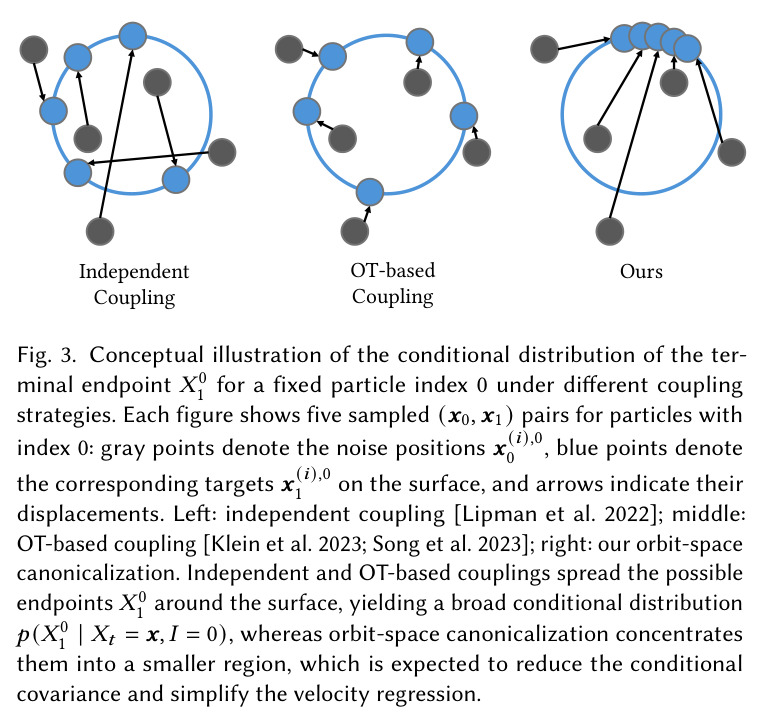
Conceptual illustration of the conditional distribution of the terminal endpoint for a fixed particle index 0 under different coupling X_0,1 strategies. Each figure shows five sampled (x_0, x_1) pairs for particles with index 0.
Fig. 3: Conceptual illustration of the conditional distribution of the terminal endpoint for a fixed particle index 0 under different coupling X_0,1 strategies. Each figure shows five sampled (x_0, x_1) pairs for particles with index 0.
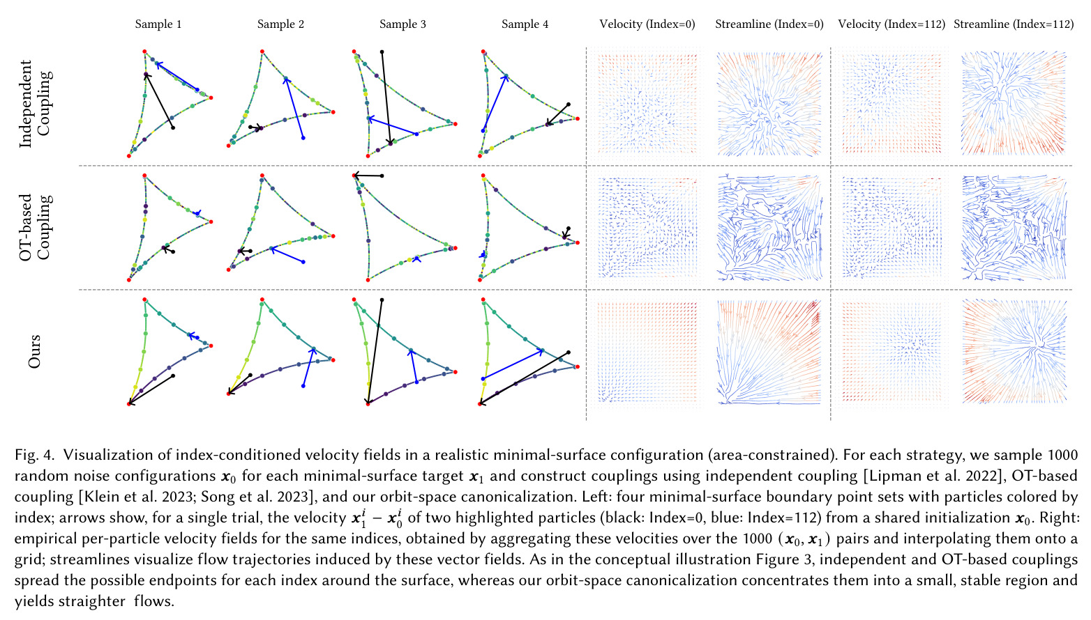
Visualization of index-conditioned velocity fields in a realistic minimal-surface configuration (area-constrained). For each strategy, we sample 1000 random noise configurations x_0 for each minimal-surface target x_1 and construct couplings using independent coupling, OT-based coupling, and our orbit-space canonicalization.
Fig. 4: Visualization of index-conditioned velocity fields in a realistic minimal-surface configuration (area-constrained). For each strategy, we sample 1000 random noise configurations x_0 for each minimal-surface target x_1 and construct couplings using independent coupling, OT-based coupling, and our orbit-space canonicalization.
Geometric probability paths for attribute encoding. Left: Our geometric probability path (quadratic Hermite curve) aligns the terminal tangent with the surface normal n_1, encoding per-particle attributes into the path geometry. Right: Standard linear interpolation leaves the terminal velocity as an unused degree of freedom.
Fig. 8: Geometric probability paths for attribute encoding. Left: Our geometric probability path (quadratic Hermite curve) aligns the terminal tangent with the surface normal n_1, encoding per-particle attributes into the path geometry. Right: Standard linear interpolation leaves the terminal velocity as an unused degree of freedom.
Comparison of terminal velocity magnitude choices. Red dots indicate uniform time samples t in {0, 0.2, 0.4, 0.6, 0.8, 1.0}; green arrows show v_1. Top: NTV sets ||v_1|| = 1, yielding nonuniform arc-length spacing. Middle: Our ATV approximation sets ||v_1|| = D(1 + lambda(1 - S)), achieving near-uniform spacing with negligible overhead. Bottom: Numerically optimized ATV chooses ||v_1|| to minimize speed variance along the curve, giving optimal uniformity but requiring numerical optimization.
Fig. 10: Comparison of terminal velocity magnitude choices. Red dots indicate uniform time samples t in {0, 0.2, 0.4, 0.6, 0.8, 1.0}; green arrows show v_1. Top: NTV sets ||v_1|| = 1, yielding nonuniform arc-length spacing. Middle: Our ATV approximation sets ||v_1|| = D(1 + lambda(1 - S)), achieving near-uniform spacing with negligible overhead. Bottom: Numerically optimized ATV chooses ||v_1|| to minimize speed variance along the curve, giving optimal uniformity but requiring numerical optimization.
Mid-time analysis of Lipschitz ratios and directional cancellation. From left to right: median and 90th percentile Lipschitz ratio, median and 90th percentile cancellation score at t=1/2 over k-NN edges (bins ordered by distance). Lower L_ij and higher s_canc are better. Canonicalizing X_1 only ('sort x_1', Ours) yields the lowest Lipschitz ratios and highest cancellation scores, matching our directional-cancellation analysis.
Fig. 28: Mid-time analysis of Lipschitz ratios and directional cancellation. From left to right: median and 90th percentile Lipschitz ratio, median and 90th percentile cancellation score at t=1/2 over k-NN edges (bins ordered by distance). Lower L_ij and higher s_canc are better. Canonicalizing X_1 only ('sort x_1', Ours) yields the lowest Lipschitz ratios and highest cancellation scores, matching our directional-cancellation analysis.

实验结果

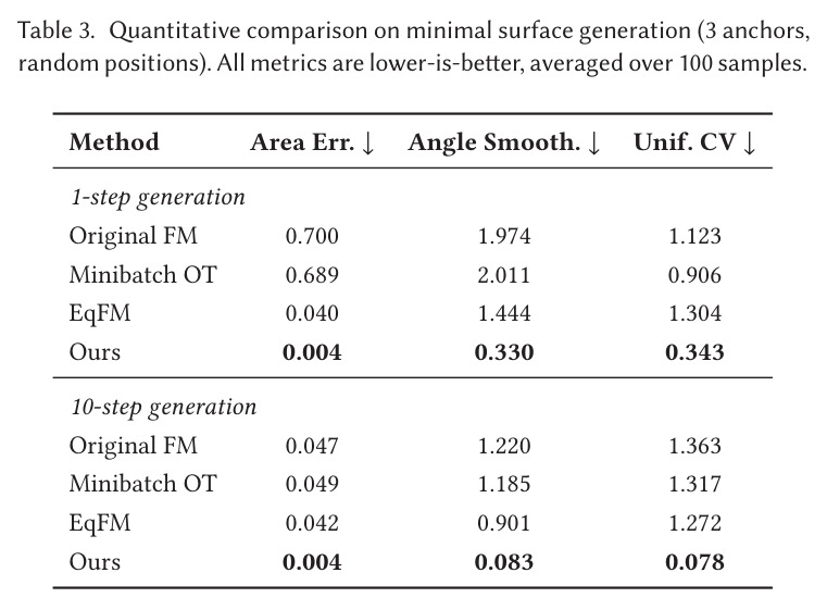
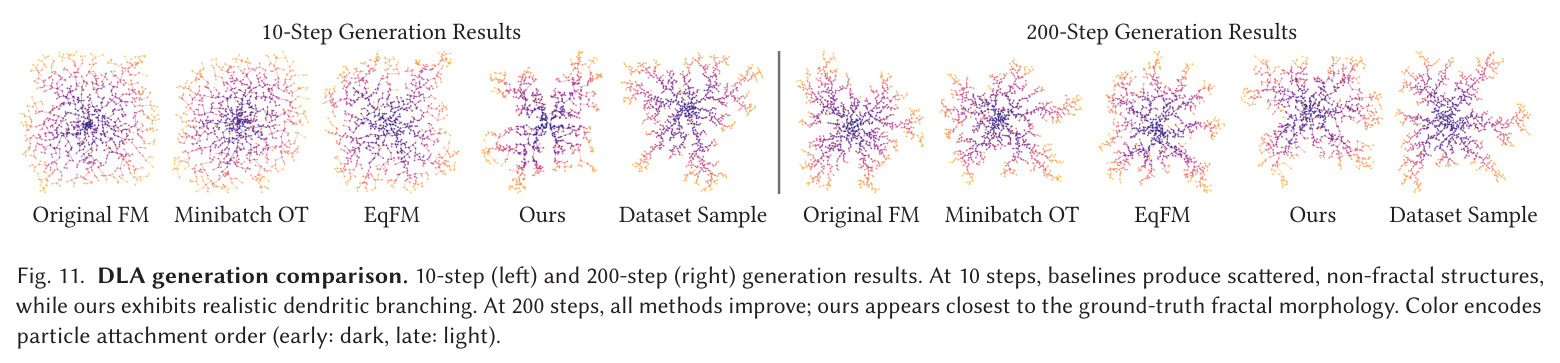
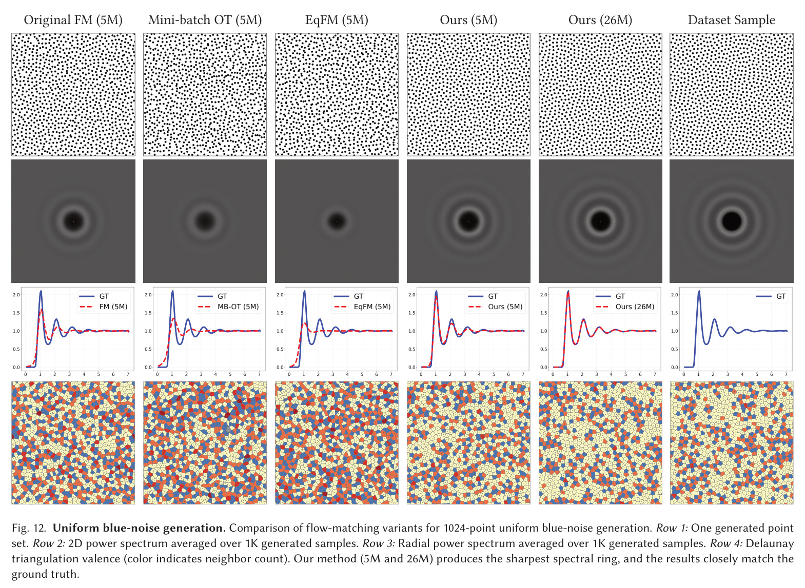
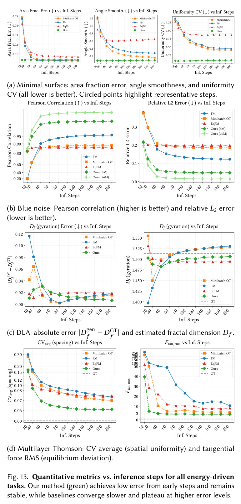
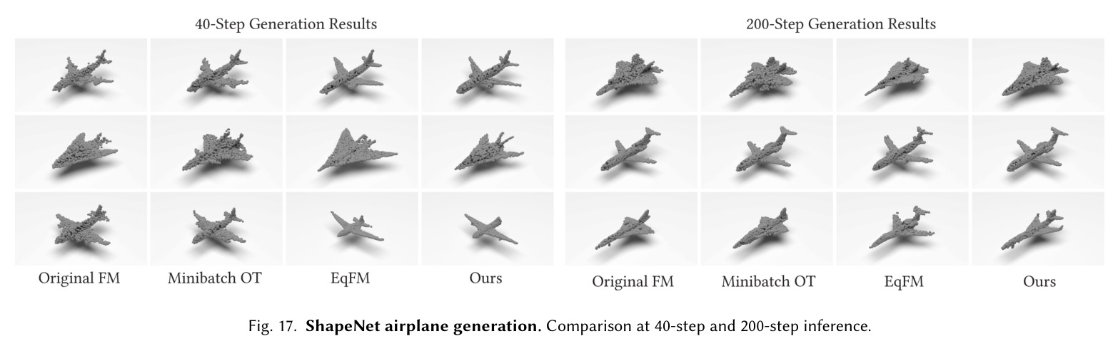
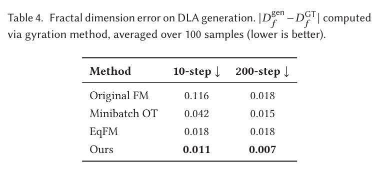
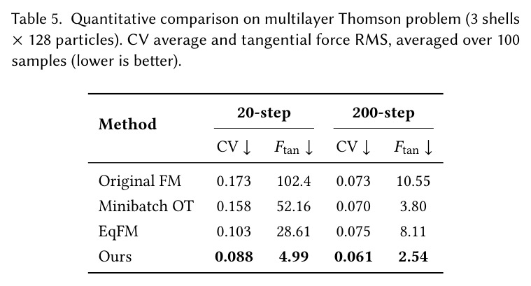
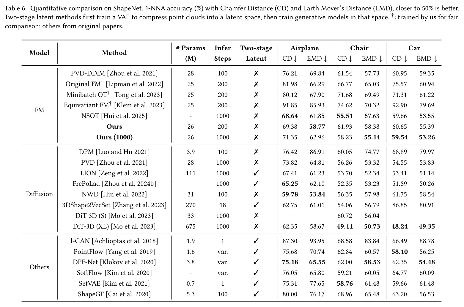
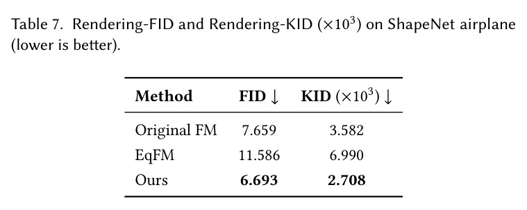
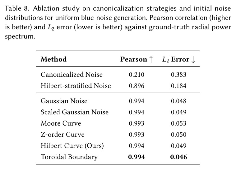
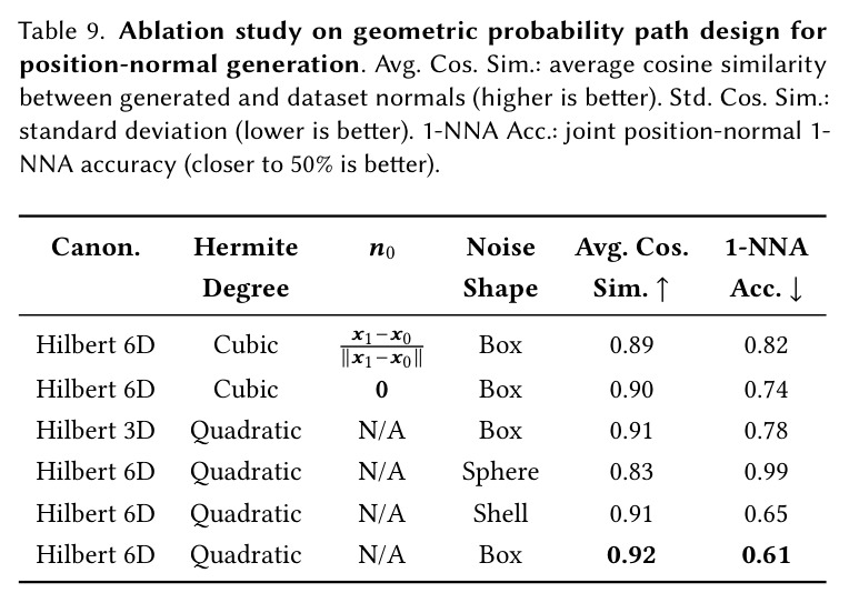
OGPP 在四类能量驱动粒子生成任务和两类 3D 形状生成任务上一致达到 SOTA 或匹配 SOTA。在蓝噪声生成 (1024 点) 上,5M 参数模型相对 Original Flow Matching (Pearson 0.956, $L_2$ 0.122) 取得 Pearson 0.994 和 $L_2$ 0.049,26M 大模型更达到 Pearson 0.999 和 $L_2$ 0.014,而 EqFM 仅 0.867 和 0.198。在最小曲面生成 (3 锚点) 这一最具挑战性的条件任务上,单步推理即达到面积误差 0.004、角度平滑度 0.330、均匀度 CV 0.343,比 Original FM (0.700/1.974/1.123) 和 Minibatch OT (0.689/2.011/0.906) 提升近两个数量级;10 步时进一步降到 0.004/0.083/0.078,所有指标都比 EqFM (0.042/0.901/1.272) 好一个数量级,且从图 Figure 13a 看基线即使 200 步都收敛不到这个水平。在 DLA 分形生成上,10 步分形维数误差 0.011 (Original FM 0.116、EqFM 0.018),200 步 0.007 (基线 0.015–0.018);在多层 Thomson 三球壳 × 128 粒子问题上,20 步切向力 RMS 4.99 (Original FM 102.4),200 步 2.54 (基线 3.80–10.55),表明生成配置接近真正的能量极小解。在 ShapeNet 三个类别上 (Table 6),26M 模型的 EMD 全面优于其他 flow matching 基线:飞机 58.77、椅子 58.38、汽车 55.39;飞机 EMD 58.77 与 DiT-3D XL (675M 参数、1000 步) 的 58.67 几乎相当,但用 26 倍少参数 + 5 倍少步数;NSOT 在 1000 步达 61.85 飞机 EMD,OGPP 仅用 200 步就达到 58.77。ShapeNet 飞机 Rendering-FID/KID 上 OGPP 取得 6.693/2.708×10³,优于 Original FM (7.659/3.582×10³) 和 EqFM (11.586/6.990×10³)。单形状编码 (Thingi10k) 上 ATV 中位无向角度误差 7.6° vs PCA-ATV 12.4°、NTV 10.9° vs PCA-NTV 17.3°,且 ATV 与 6D 直接生成方法质量相当但仅用 3D 表示。Ablation 还揭示几个关键设计点:仅规范化 $X_0$ 而不规范 $X_1$ 时 Pearson 暴跌到 0.21,与理论一致;6D Hilbert 比 3D Hilbert 把 1-NNA 从 0.78 改善到 0.61;quadratic 比 cubic Hermite 表现更好;box noise 比 sphere/shell noise 更好 (1-NNA 0.61 vs 0.99)。
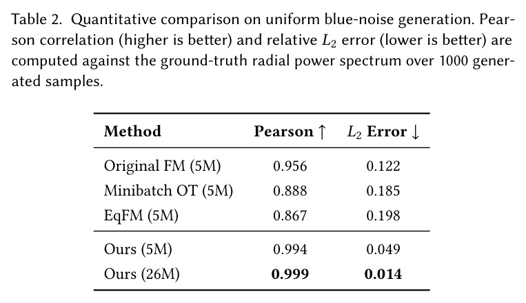
Quantitative comparison on uniform blue-noise generation. Pearson correlation and relative L2 error computed against the ground-truth radial power spectrum over 1000 generated samples.
Table 2: Quantitative comparison on uniform blue-noise generation. Pearson correlation and relative L2 error computed against the ground-truth radial power spectrum over 1000 generated samples.
Quantitative comparison on minimal surface generation (3 anchors, random positions). All metrics are lower-is-better, averaged over 100 samples.
Table 3: Quantitative comparison on minimal surface generation (3 anchors, random positions). All metrics are lower-is-better, averaged over 100 samples.
Quantitative comparison on ShapeNet. 1-NNA accuracy (%) with Chamfer Distance (CD) and Earth's Mover Distance (EMD); closer to 50% is better. Two-stage latent methods first train a VAE to compress point clouds into a latent space, then train generative models in that space.
Table 6: Quantitative comparison on ShapeNet. 1-NNA accuracy (%) with Chamfer Distance (CD) and Earth's Mover Distance (EMD); closer to 50% is better. Two-stage latent methods first train a VAE to compress point clouds into a latent space, then train generative models in that space.
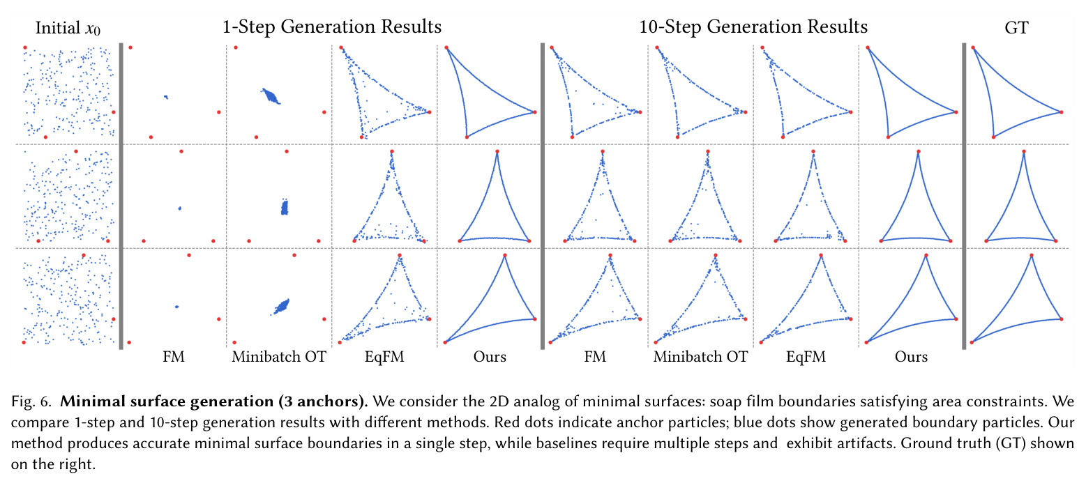
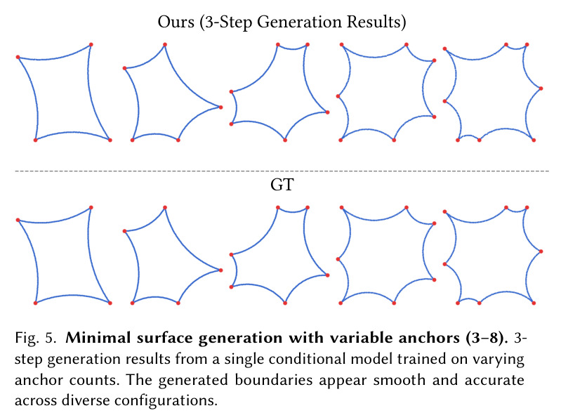
Minimal surface generation (3 anchors). We consider the 2D analog of minimal surfaces: soap film boundaries satisfying area constraints. We compare 1-step and 10-step generation results with different methods. Red dots indicate anchor particles; blue dots show generated boundary particles. Our method produces accurate minimal surface boundaries in a single step, while baselines require multiple steps and exhibit artifacts.
Fig. 6: Minimal surface generation (3 anchors). We consider the 2D analog of minimal surfaces: soap film boundaries satisfying area constraints. We compare 1-step and 10-step generation results with different methods. Red dots indicate anchor particles; blue dots show generated boundary particles. Our method produces accurate minimal surface boundaries in a single step, while baselines require multiple steps and exhibit artifacts.
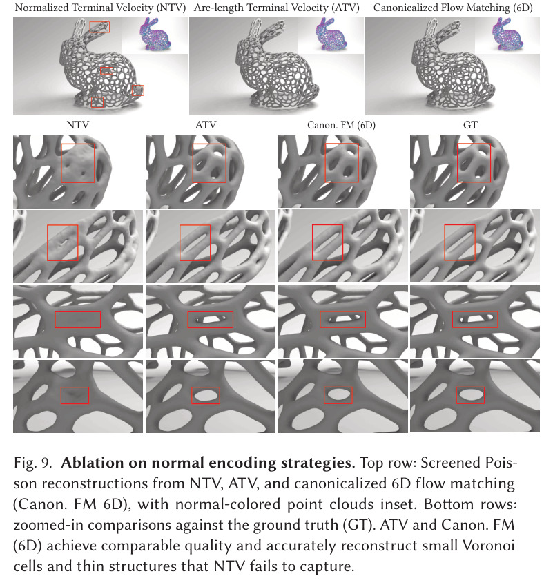
Ablation on normal encoding strategies. Top row: Screened Poisson reconstructions from NTV, ATV, and canonicalized 6D flow matching (Canon. FM 6D), with normal-colored point clouds inset. Bottom rows: zoomed-in comparisons against the ground truth (GT). ATV and Canon. FM (6D) achieve comparable quality and accurately reconstruct small Voronoi cells and thin structures that NTV fails to capture.
Fig. 9: Ablation on normal encoding strategies. Top row: Screened Poisson reconstructions from NTV, ATV, and canonicalized 6D flow matching (Canon. FM 6D), with normal-colored point clouds inset. Bottom rows: zoomed-in comparisons against the ground truth (GT). ATV and Canon. FM (6D) achieve comparable quality and accurately reconstruct small Voronoi cells and thin structures that NTV fails to capture.
DLA generation comparison. 10-step (left) and 200-step (right) generation results. At 10 steps, baselines produce scattered, non-fractal structures, while ours exhibits realistic dendritic branching. At 200 steps, all methods improve; ours appears closest to the ground-truth fractal morphology. Color encodes particle attachment order (early: dark, late: light).
Fig. 11: DLA generation comparison. 10-step (left) and 200-step (right) generation results. At 10 steps, baselines produce scattered, non-fractal structures, while ours exhibits realistic dendritic branching. At 200 steps, all methods improve; ours appears closest to the ground-truth fractal morphology. Color encodes particle attachment order (early: dark, late: light).
Uniform blue-noise generation. Comparison of flow-matching variants for 1024-point uniform blue-noise generation. Row 1: One generated point set. Row 2: 2D power spectrum averaged over 1K generated samples. Row 3: Radial power spectrum averaged over 1K generated samples. Row 4: Delaunay triangulation valence (color indicates neighbor count). Our method (5M and 26M) produces the sharpest spectral ring, and the results closely match the ground truth.
Fig. 12: Uniform blue-noise generation. Comparison of flow-matching variants for 1024-point uniform blue-noise generation. Row 1: One generated point set. Row 2: 2D power spectrum averaged over 1K generated samples. Row 3: Radial power spectrum averaged over 1K generated samples. Row 4: Delaunay triangulation valence (color indicates neighbor count). Our method (5M and 26M) produces the sharpest spectral ring, and the results closely match the ground truth.
Quantitative metrics vs. inference steps for all energy-driven tasks. Our method (green) achieves low error from early steps and remains stable, while baselines converge slower and plateau at higher error levels.
Fig. 13: Quantitative metrics vs. inference steps for all energy-driven tasks. Our method (green) achieves low error from early steps and remains stable, while baselines converge slower and plateau at higher error levels.
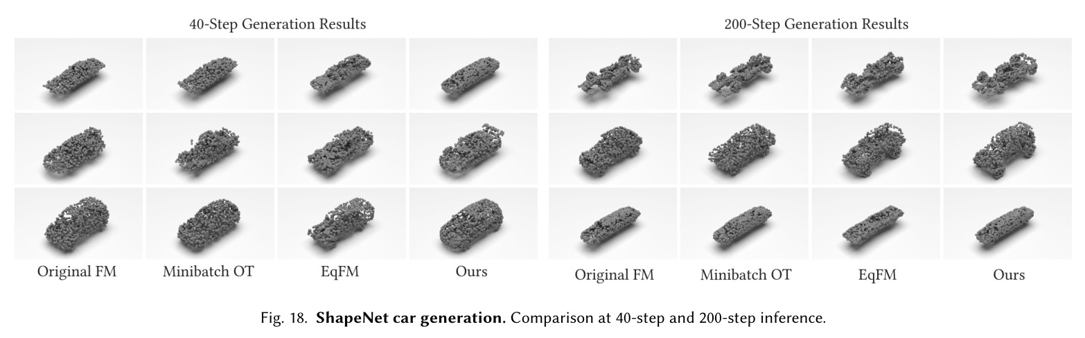
ShapeNet airplane generation. Comparison at 40-step and 200-step inference.
Fig. 17: ShapeNet airplane generation. Comparison at 40-step and 200-step inference.
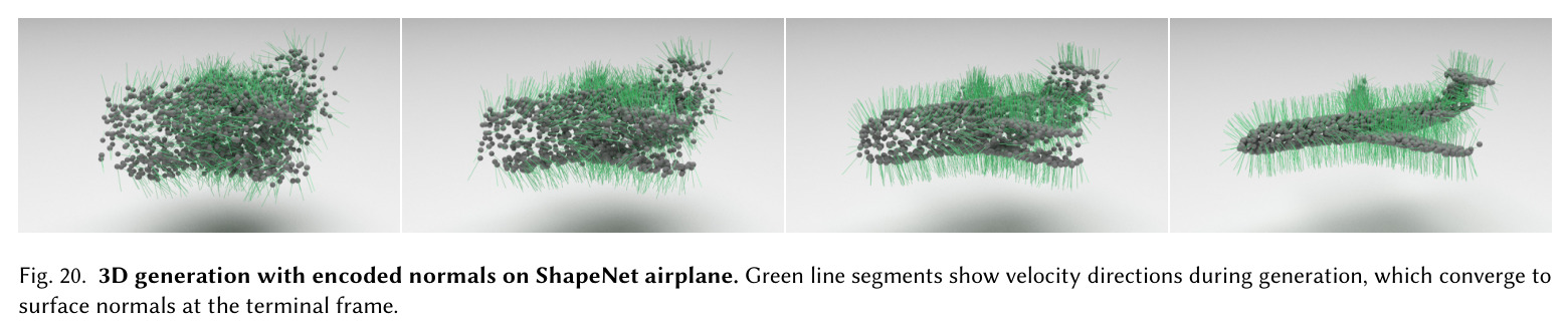
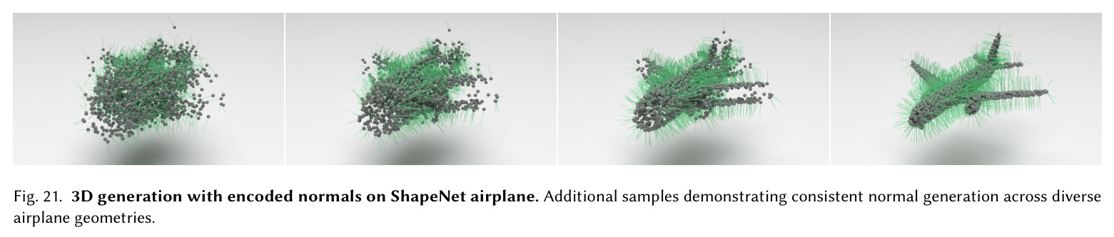
3D generation with encoded normals on ShapeNet airplane. Green line segments show velocity directions during generation, which converge to surface normals at the terminal frame.
Fig. 20: 3D generation with encoded normals on ShapeNet airplane. Green line segments show velocity directions during generation, which converge to surface normals at the terminal frame.
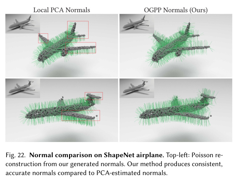
Normal comparison on ShapeNet airplane. Top-left: Poisson reconstruction from our generated normals. Our method produces consistent, accurate normals compared to PCA-estimated normals.
Fig. 22: Normal comparison on ShapeNet airplane. Top-left: Poisson reconstruction from our generated normals. Our method produces consistent, accurate normals compared to PCA-estimated normals.
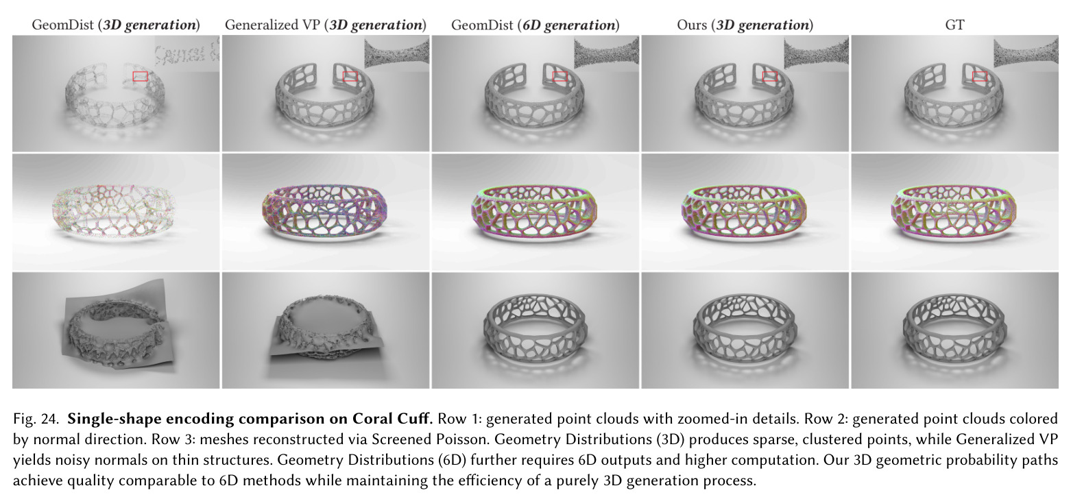
Single-shape encoding comparison on Coral Cuff. Row 1: generated point clouds with zoomed-in details. Row 2: generated point clouds colored by normal direction. Row 3: meshes reconstructed via Screened Poisson. Geometry Distributions (3D) produces sparse, clustered points, while Generalized VP yields noisy normals on thin structures. Geometry Distributions (6D) further requires 6D outputs and higher computation. Our 3D geometric probability paths achieve quality comparable to 6D methods while maintaining the efficiency of a purely 3D generation process.
Fig. 24: Single-shape encoding comparison on Coral Cuff. Row 1: generated point clouds with zoomed-in details. Row 2: generated point clouds colored by normal direction. Row 3: meshes reconstructed via Screened Poisson. Geometry Distributions (3D) produces sparse, clustered points, while Generalized VP yields noisy normals on thin structures. Geometry Distributions (6D) further requires 6D outputs and higher computation. Our 3D geometric probability paths achieve quality comparable to 6D methods while maintaining the efficiency of a purely 3D generation process.
Minimal surface (area-constrained) generation ablation study (3 anchors). Comparison of 1-step and 10-step generations; red dots indicate anchor points (conditioning locations), and ground truth (GT) is shown on the right. Without per-particle index (identity) embeddings, our method has only similar expressive power to vanilla Flow Matching (Eulerian view), while equipping vanilla Flow Matching with particle identities alone still fails to produce high-quality minimal surfaces.
Fig. 25: Minimal surface (area-constrained) generation ablation study (3 anchors). Comparison of 1-step and 10-step generations; red dots indicate anchor points (conditioning locations), and ground truth (GT) is shown on the right. Without per-particle index (identity) embeddings, our method has only similar expressive power to vanilla Flow Matching (Eulerian view), while equipping vanilla Flow Matching with particle identities alone still fails to produce high-quality minimal surfaces.
查看结构化数据
任务指标本文基线提升
Uniform Blue-Noise Generation (1024 points) Pearson correlation (radial power spectrum) 0.999 (26M) / 0.994 (5M) Original FM 0.956 / EqFM 0.867 / Minibatch OT 0.888 +4.3% (vs Original FM), +15.2% (vs EqFM)
Uniform Blue-Noise Generation (1024 points) Relative L2 error 0.014 (26M) / 0.049 (5M) Original FM 0.122 / EqFM 0.198 约 9 倍降低 (vs Original FM),约 14 倍降低 (vs EqFM)
Minimal Surface Generation (3 anchors, 1-step) Area Fraction Error 0.004 Original FM 0.700 / Minibatch OT 0.689 / EqFM 0.040 提升 10-175 倍
Minimal Surface Generation (3 anchors, 10-step) Area Fraction Error 0.004 Original FM 0.047 / EqFM 0.042 提升 10 倍以上
DLA Fractal Dimension (gyration method, 10-step) |D_f^gen - D_f^GT| 0.011 Original FM 0.116 / Minibatch OT 0.042 / EqFM 0.018 约 10 倍降低 (vs Original FM),约 1.6 倍降低 (vs EqFM)
DLA Fractal Dimension (gyration method, 200-step) |D_f^gen - D_f^GT| 0.007 Original FM 0.018 / Minibatch OT 0.015 / EqFM 0.018 约 2 倍降低
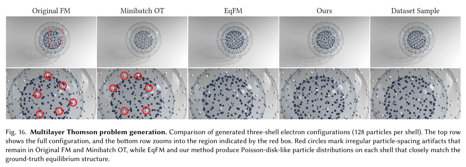
Multilayer Thomson Problem (3 shells × 128 particles, 20-step) Tangential Force RMS 4.99 Original FM 102.4 / Minibatch OT 52.16 / EqFM 28.61 约 6-20 倍降低
Multilayer Thomson Problem (3 shells × 128 particles, 200-step) Tangential Force RMS 2.54 Original FM 10.55 / Minibatch OT 3.80 / EqFM 8.11 1.5-4 倍降低
ShapeNet Airplane (2048 points) 1-NNA EMD (%) 58.77 (200-step), 62.96 (1000-step) DiT-3D XL 58.67 (1000-step, 675M params) / NSOT 61.85 (1000-step) 匹配 DiT-3D XL 用 26× 少参数 + 5× 少步;匹配 NSOT 用 5× 少步
ShapeNet Airplane Rendering-FID FID (lower better) 6.693 Original FM 7.659 / EqFM 11.586 FID 降低 12.6% (vs Original FM),42% (vs EqFM)
Single-Shape Encoding Normal Accuracy (Thingi10k) Median unoriented angular error ATV 7.6° PCA-ATV 12.4° / NTV 10.9° / PCA-NTV 17.3° 角度误差降低约 30-56%

局限与改进

作者明确承认四点局限:(1) 当前框架要求固定粒子数 $N$,且依赖 full attention,对粒子数的二次方复杂度限制了大粒子系统扩展性;(2) 几何概率路径不具备 Wasserstein-2 位移插值的测地线性质 (W2 geodesics),可能引入稍微弯曲的概率流;(3) 规范化只利用了'输出稳定索引'这一性质,没有把索引结构本身 (如排序、局部性) 作为额外信息通道编码到任务相关语义中;(4) 当数据集样本间共享结构较少时规范化收益会减弱——在合成基准 (最小曲面、蓝噪声) 上提升巨大,而在复杂真实形状 (多样 ShapeNet 类别) 上提升较温和。从我自己的观察还可以补充:(5) 单边规范化的选择虽在 Lipschitz 比上最优,但条件任务 (如最小曲面需要锚点排序) 与无条件任务的最优规范化策略可能不同,文章没给出统一策略;(6) ATV 公式依赖单一超参 $\lambda$,不同任务的最优 $\lambda$ 没系统给出;(7) 把表面法向编码进终端切向的'副产品'式设计依赖 $t=1$ 时条件分布塌缩到 delta 的假设,对高度各向异性或自交叉形状可能不稳定;(8) 26M 模型比 NSOT 更高效但训练 50K epoch 在 ShapeNet 上的算力代价文章未明确报告。

独立分析的弱点

独立分析几个具体弱点和改进方向:(1) **固定粒子数瓶颈**:当前所有实验都用 fixed $N$ (蓝噪声 1024、最小曲面 256、Thomson 384、ShapeNet 2048),但真实粒子系统 (流体 SPH、可变形体 MPM) 的粒子数随时间和空间变化。可考虑借鉴 Diffusion Transformer 的 patch 化或 Point Transformer V3 的窗口注意力,把 full attention 替换为空间局部注意力,并设计 hierarchical token pool 让 $N$ 可变。(2) **规范化与真实对称的耦合问题**:规范化只利用了'同构配置排到同一位置'的好处,但真实物理中的粒子身份可能本身有意义 (如分子中的不同原子类型、带电 vs 中性),强行规范化会丢失这一层信息。可以引入'软规范化'——给定一个先验相似度矩阵,仅在结构等价粒子之间做置换,而不是硬性全局排序。(3) **路径的非 W2 几何性**:Hermite 路径虽然能编码属性但不是最优传输流,最小曲面这种'面积极值'问题在 W2 意义上可能反而有更优解。可以把路径参数化推广到包含 W2 straight flow 的混合族,按任务切换。(4) **ATV 超参 $\lambda$ 的鲁棒性**:$\lambda$ 控制弧长匀速的强度,文章没给出调参准则。可以让 $\lambda$ 变成可学习的标量场,或通过离线速度方差最优化得到每粒子自适应值。(5) **索引嵌入的初始化敏感**:和 Transformer 位置编码一样,$e_i$ 的初始化方式会影响早期训练的稳定性,可以实验 sin-cos 预训练 + 微调或 random Fourier features。(6) **推理时 ODE 求解器选择**:文章没系统比较 RK4 / Dopri5 / Euler 对最终质量的影响,对 few-step 生成来说求解器选择可能比模型本身更重要。(7) **端到端可微的下游任务**:把 OGPP 生成的粒子直接喂给下游物理仿真时,需要保证生成过程是 differentiable 的,目前 ODE 积分需要 adjoint method,效率可能不佳。

未来方向

基于论文成果可延伸几个方向:(1) 作者明确提出用稀疏、分层、局部感知的架构替代 full attention,借鉴物理交互的稀疏性 (只有邻近粒子相互作用) 设计 sparse attention mask。(2) 扩展到可变粒子数:可以通过 hierarchical tokenization 或 progressive growing 实现不同尺度的粒子系统。(3) 探索更高阶或分段光滑的几何概率路径族,权衡几何属性编码与 W2 输运最优性,可以设计包含 cubic Hermite + straight segment 的混合路径。(4) 把规范化当成显式的信息通道:设计'语义感知'的规范化器 (如按 DLA 附着时间排序、按 articulated shape 关节顺序排序),让索引顺序本身编码时间或解剖学信息。(5) 把 OGPP 与下游物理仿真耦合,做'生成即仿真'的端到端 pipeline。(6) 把几何概率路径推广到编码其他属性 (曲率、密度、张量),而非仅法向。(7) 探索 continuous-time canonicalization (learned canonicalizer),替代手工 Hilbert 曲线,可能进一步压缩条件协方差。(8) 与 Rectified Flow、Reflow 等 trajectory straightening 技术结合,看能否进一步减少步数。(9) 借鉴 SGFM 的空间群对称条件扩展到晶体结构生成,把 OGPP 推向材料科学领域。

复现评估

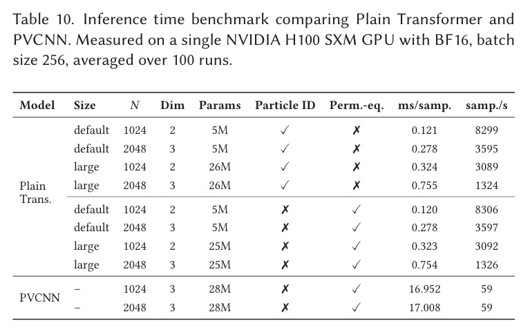
论文的复现性较好但有一定门槛。算法层面,作者给出了完整的 Algorithm 1 (训练) 和 Algorithm 2 (推理),Hermite 路径、ATV 缩放、Hilbert 排序都是确定性可复现的。模型架构是 plain Transformer encoder,代码量不大。算力需求:5M 模型在 RTX 4090 / H200 SXM 上训练 3K–8K epoch (ShapeNet 50K epoch),26M 模型用更大 batch (蓝噪声 3360),3D ShapeNet 任务算力中等。数据集方面,能量驱动任务的数据集都由论文自己生成 (蓝噪声 50K/400K 用 GBN 算法、最小曲面用 Israelachvili 近似法、DLA 用标准随机游走模拟、Thomson 用基于梯度的库仑优化),代码和数据生成脚本大概率公开 (ACM TOG 论文通常会附带项目页)。最大复现障碍是:(1) Hilbert 曲线排序和 6D 联合规范化的实现细节需要仔细处理 (Skilling 2004 的编程 Hilbert 曲线要保证 locality-preserving);(2) ATV 中 $\lambda$ 的最优值对每个任务可能不同;(3) ShapeNet 50K epoch 训练时间较长;(4) EqFM 的 OT coupling $O(B^2N^3)$ 复现成本本身就高。整体评估难度:**中等偏难**,适合有一定 flow matching 基础的研究组复现。