基于弹性测试时训练的高速空间记忆模型 Fast Spatial Memory with Elastic Test-Time Training
用弹性权重巩固稳定长序列快速权重,在 4D 重建中把 LaCT 从单块扩展到多块
前置知识
测试时训练 / TTT
一种让模型参数在推理阶段继续更新的范式。与固定权重的常规推理不同,TTT 在每个测试样本上对一部分参数(称为快速权重)做梯度下降,使其从当前上下文中学到任务相关的关联。在本文中 TTT 层用一个小网络 $f_\theta$ 把第 $i$ 个 token 的 key $k_i$ 变换后逼近对应的 value $v_i$,目标是最小化 $L(f_\theta(k_i), v_i)$。
TTT 是 LaCT 以及本文 LaCET 的直接前身。要理解 LaCET 为什么要引入 EWC 正则项,必须先理解 TTT 的 update/apply 双操作和快速权重的概念。
大块测试时训练 / LaCT
LaCT 把 TTT 的逐 token 更新改成逐 chunk 更新:把长度为 $N$ 的输入切成 $C$ 个块,每个块共享同一组快速权重,先对整个块的 KV 统计量做一次 surrogate 更新 $ \theta_{c+1}=\theta_c-\eta\nabla_\theta\sum_{i=1}^{b} L(f_\theta(k_i), v_i)$,再用更新后的权重处理该块所有 query。
LaCT 是 LaCET 的起点。LaCET 完全沿用 LaCT 的 chunk-wise 公式,但额外加了一个 'consolidate' 步骤去缓解 LaCT 快速权重在长序列上的过拟合和漂移。
弹性权重巩固 / EWC
EWC 是 continual learning 中防止灾难性遗忘的方法。它把对旧任务重要的参数用 Fisher 信息矩阵 $F$ 标定出来,对这些参数加二次惩罚 $\lambda \sum_i F_i (\theta_i-\theta^*_i)^2$,把它们拉回 anchor $\theta^*$。在本文中 Fisher 矩阵被改成在 chunk 边界上用 EMA 累积。
EWC 的核心思想被直接搬到了测试时:把上一个 chunk 的快速权重当成旧任务 anchor,再去稳定新 chunk 的更新。这是 LaCET 区别于 LaCT 的关键。
Plücker 射线图
Plücker 坐标用 6 维向量同时编码光线的方向和位置 $(r_d, r_o \times r_d)$,其中 $r_d$ 是方向、$r_o$ 是射线原点。把这个 6 维图与 RGB 拼接成 9 通道,再叠上一个时间戳通道形成 10 通道的输入特征图,可以把相机几何直接注入视觉 token。
FSM 用 Plücker 图作为几何增强,使同一组 token 能在不同视角和时间下区分开,是实现 pose-conditioned 4D NVS 的关键。
研究动机
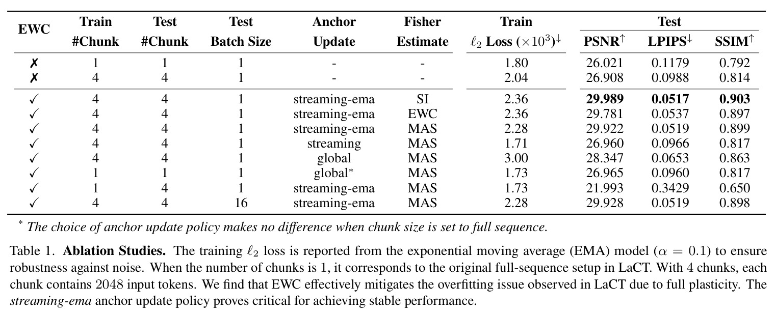
当前主流的 3D/4D 重建大模型(如 LRM、LVSM、tttLRM)几乎都建立在 Transformer 的自回归或全注意力之上,激活显存随上下文长度线性增长,序列稍微变长就放不下。LaCT 通过把 TTT 改成 chunk-wise 大幅降低了显存,但它的快速权重在推理时是'完全可塑'的——每个 chunk 都会沿着梯度方向自由漂移。在 4D 场景里,光照、相机姿态、物体运动随时间不断变化,连续多次全塑性更新会让快速权重偏离合理区域,表现为训练-测试 PSNR 差距巨大、出现重影、相机姿态插值走捷径(只会在相邻帧之间做插值,而学不会真正的 NVS)。作者在 Stereo4D 上一组消融实验中明确测到 LaCT(4 chunks)的训练 $\ell_2$ 损失只有 2.04,而测试 PSNR 只有 26.908;引入 EWC 后,训练损失虽上升到 2.36 但测试 PSNR 跳到 29.989,差距被显著缩小。这说明 LaCT 的瓶颈不是容量而是稳定性。
本文的目标是本文目标有两个层面。架构层面:把 LaCT 从 '单块 + 完全可塑' 升级为 '多块 + 弹性可塑',使模型能在激活显存可控的前提下处理任意长度的输入-时间序列。系统层面:在升级后的 LaCET 之上预训练一个真正的 4D 大模型 FSM,使其能在任意 (view, time) 组合下渲染出与训练时序一致、几何合理的新视角,并且在 3D NVS 基准(DL3DV)上不输给纯静态模型。
与已有工作不同的是,已有方案可以大致分成三类:长上下文注意力类(Long-LRM++、LoGeR)通过状态空间或 hybrid 注意力延长序列,但仍是静态 3D;TTT 类(tttLRM、ttt3R、LaCT)虽然把 4D 拉进来,但都是单块或全塑性;EWC 类算法只在 offline continual learning 里用过。本文把 EWC 改造成 'chunk 边界的弹性先验',并把它和 LaCT 的 chunk-wise 公式无缝拼起来,是首个把 '快速权重的稳定性' 显式引入 4D 重建的工作。
核心方法
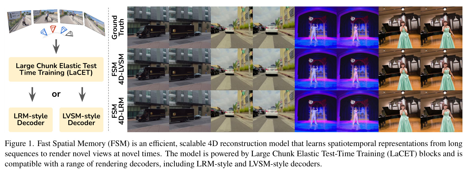
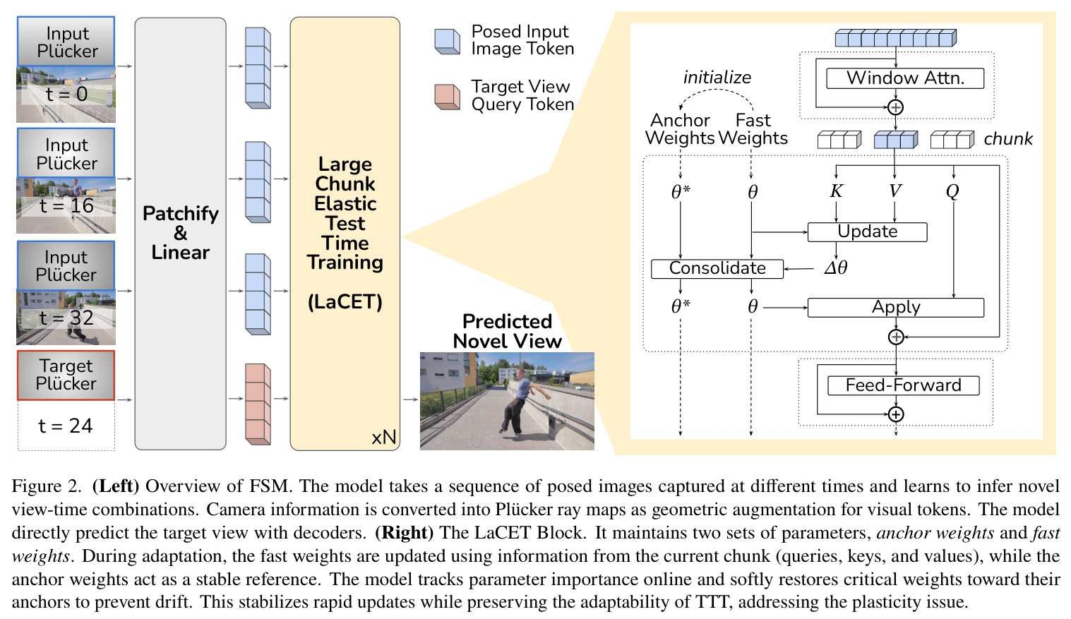
FSM 的整体思路是:先把 $V$ 张带 pose 的图像 patchify 成视觉 token,再叠上 Plücker 射线图和时间戳,让同一组 token 携带几何与时间信息;然后把这些 token 丢进一摞 LaCET 块。LaCET 块的快速权重是单头 SwiGLU MLP,对每个 chunk 内的 key/value 用自监督损失做一次 surrogate 梯度更新,再用同样的权重处理 target query;为了避免更新漂移,块内还维护一组 anchor 权重(按 streaming-EMA 演化)和一份 Fisher 重要性矩阵,update 之后用一个 EWC 风格的二次项把 '重要' 参数拉回 anchor。最后在输出端用两个 decoder 之一(LVSM 风格的线性 RGB head,或 LRM 风格的 4D Gaussian Splatting head)把 token 还原成目标视角图像。
核心创新是在 LaCT 的 update 之后新增一个 consolidate 算子 $\theta_{c+1}=\theta'_c - \lambda F_c \odot (\theta'_c - heta^*_c)$,把上一个 chunk 的快速权重当成 '旧任务',再用 Fisher 加权的二次正则把新 chunk 的更新约束在 anchor 附近;同时把 anchor 改成 streaming-EMA $\theta^* \leftarrow \beta\theta^* + (1-\beta)\theta$。这与 LaCT 的本质区别是:LaCT 让快速权重在每块之间完全自由漂移,LaCET 让漂移被一个低通的、自适应的弹簧抑制。配合三种 Fisher 估计(EWC、MAS、SI),作者在 Stereo4D 消融里证明 streaming-EMA + MAS 把 4-chunk 设置的 PSNR 从 26.908 提到 29.928,把 $\ell_2$ 测试损失压到 1.71。
方法步骤详情
方法分四步。第一步是图像 token 化:每张输入 $I_j \in \mathbb{R}^{H\times W\times 3}$ 与对应 Plücker 射线图 $P_j$、时间戳 $T_j$ 沿通道维拼接成 10 通道 $e_{I_j}$,再 patchify 成 $p\times p$ 的 patch 并线性投影到 $D$ 维 token;目标视角则构造一份外观通道为零、pose/时间通道填充完整的 query token。第二步是 LaCET 块的前向:token 经 window attention 之后进入 SwiGLU-MLP 快速权重网络 $f_\theta$,$\theta=\{\theta_1,\theta_2,\theta_3\}$,对每个输入 chunk 内部用损失 $L(f_\theta(k_i), v_i)=-f_\theta(k_i)^\top v_i$ 做一次 surrogate 梯度更新 $\theta'_c=\theta_c-\eta\nabla_\theta\sum_{i=1}^{b}L$。第三步是 EWC 风格 consolidate:用 EMA 累积的 Fisher 矩阵 $F_{c+1}=\alpha F_c + (1-\alpha)\varphi(S_c)$ 评估参数重要性,再施加 $\theta_{c+1}=\theta'_c-\lambda F_c\odot(\theta'_c-\theta^*_c)$,并按 $\theta^*\leftarrow\beta\theta^*+(1-\beta)\theta$ 滚动 anchor。第四步是解码:FSM-LVSM 用 linear+sigmoid+unpatchify 直接从 token 还原 RGB patch;FSM-LRM 用 linear 头解出 $V\times H\times W$ 个 20 维 4D Gaussian 原语 $(\mathbf{g}_{xyz}, g_t, \mathbf{g}_{rgb}, \mathbf{g}_{scale,xyz}, g_{scale,t}, \mathbf{g}_{rot,l}, \mathbf{g}_{rot,r}, g_{opacity})$,再用 tile-based 渲染器得到目标视角。整模型用 $\ell_2$ + LPIPS 损失 $(\mu=0.5)$ 端到端训练。
技术新颖性
技术新颖性体现在三点。第一,把 EWC 从离线 continual learning 搬到流式推理:anchor 不是训练完固定的值,而是 chunk 边界上的 EMA,本质上把 EWC 变成一个低通滤波器作用于快速权重轨迹。第二,对 Fisher 估计做了系统消融(EWC/MAS/SI),并发现 MAS 在 4 块设置下表现最佳(PSNR 29.928),而 EWC 和 SI 略低(29.781/29.989,但训练损失接近),这是关于 '什么算作重要参数' 的新经验。第三,给出 chunk 切分、anchor 更新策略、batch size 影响的统一公式,使 LaCET 成为第一个 '多 chunk、弹性可塑' 的快速权重层,并在 4D 重建上让 PSNR/SSIM/LPIPS 在 32 输入帧设定下全面超过 LaCT。
实验结果
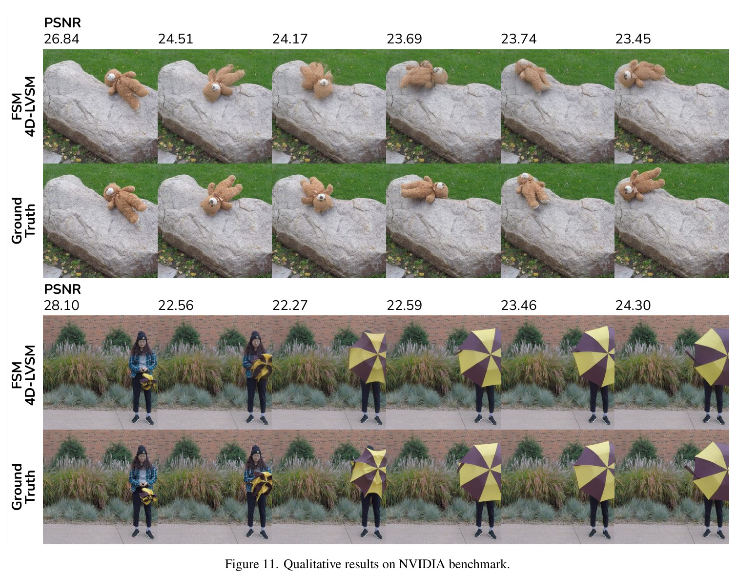
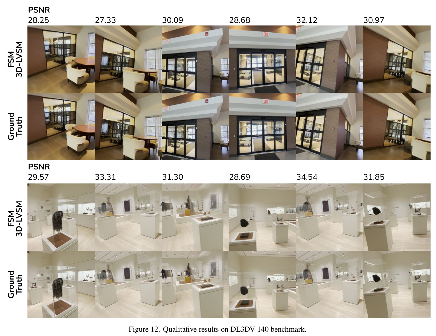
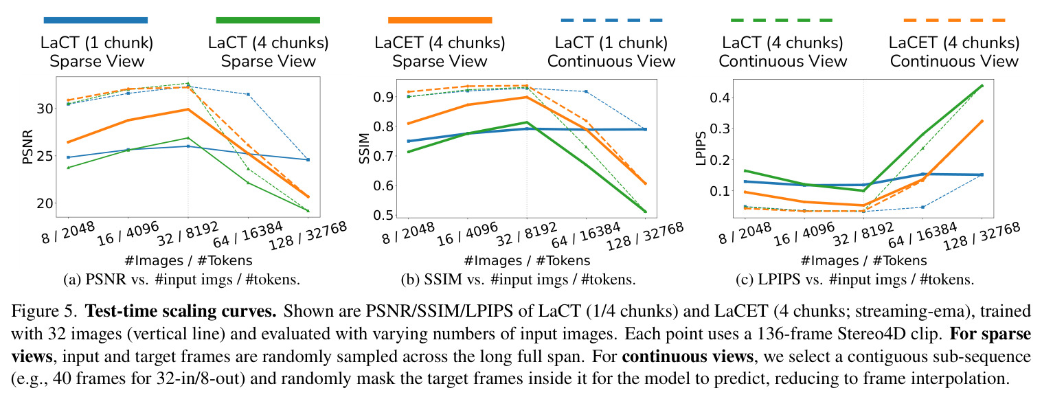
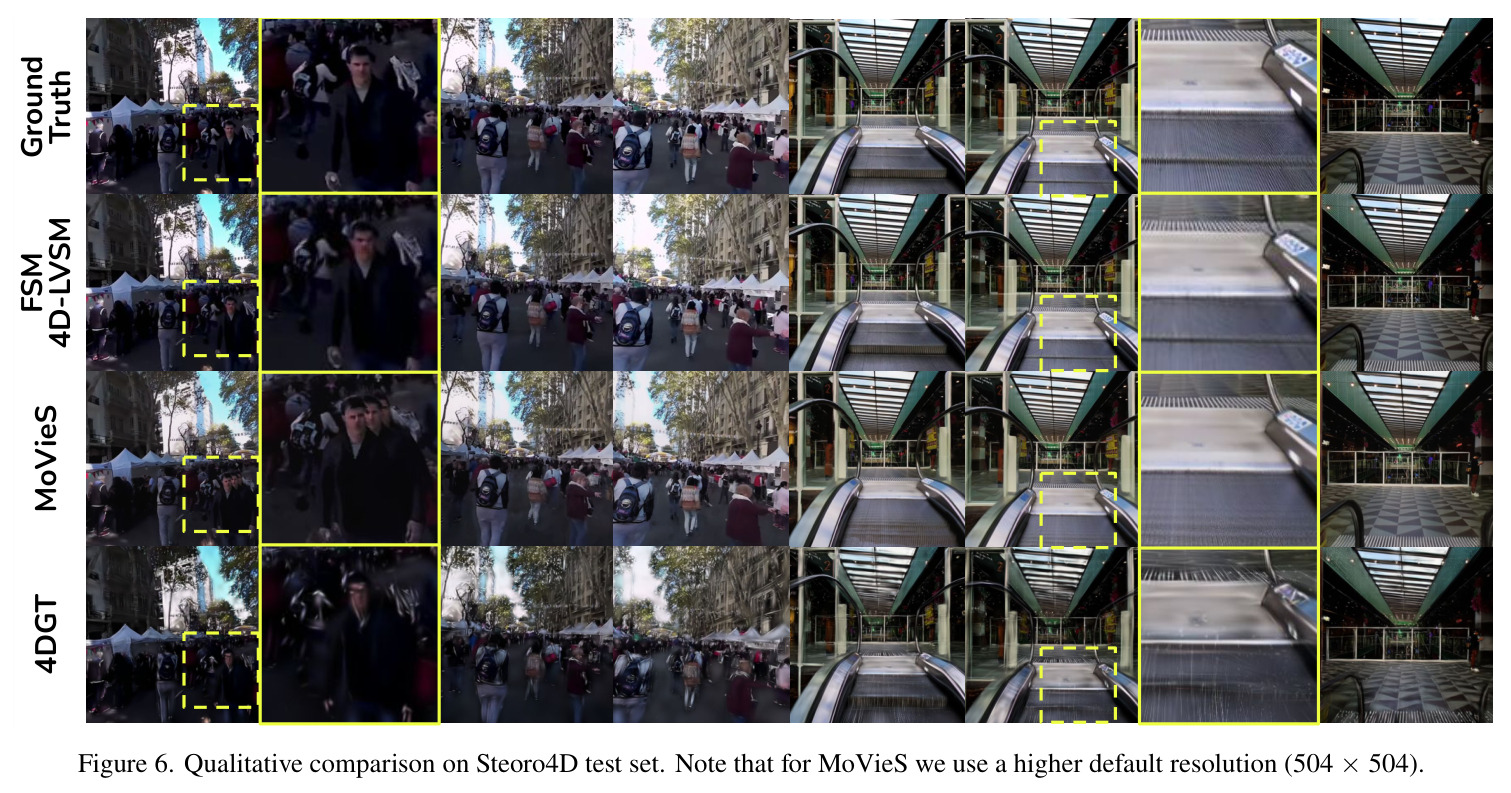
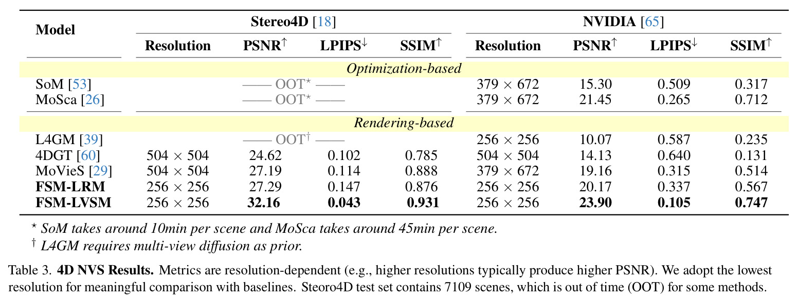
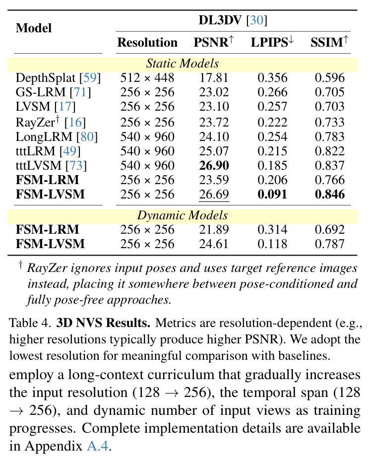
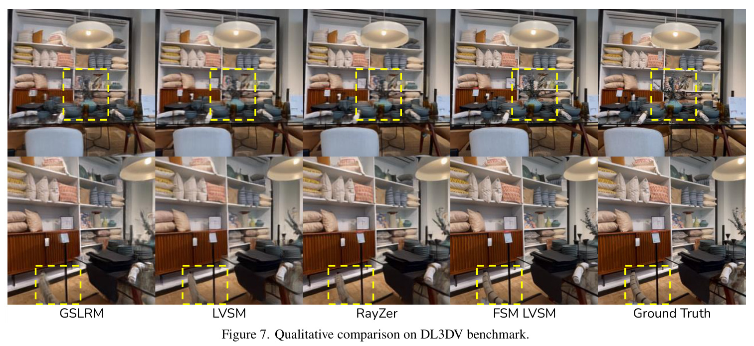
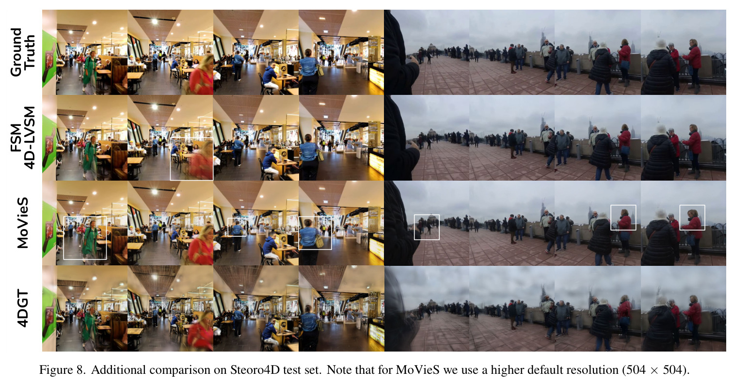
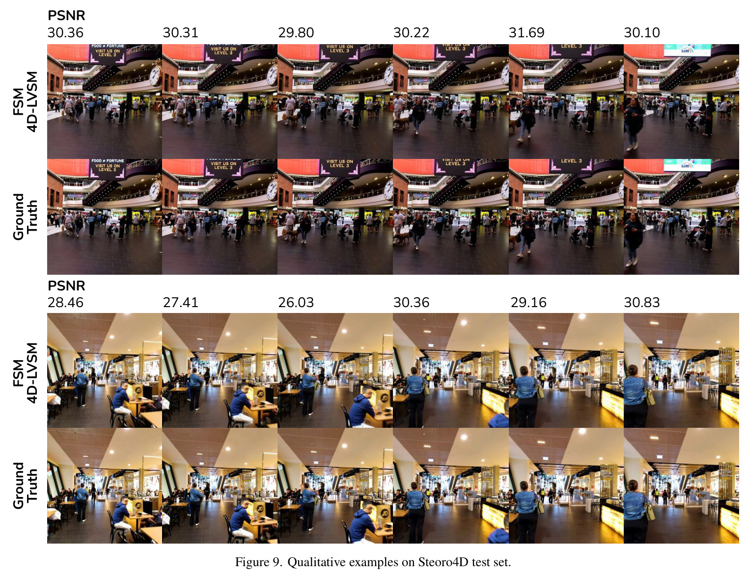
在 Stereo4D 受控消融里,作者固定 32 输入视图、128 时间窗、12 层 LaCET,结论非常清晰:单块 LaCT 测试 PSNR 26.021;切成 4 块后 LaCT 由于漂移只到 26.908;加 EWC + streaming-EMA + MAS 之后跳到 29.928,LPIPS 从 0.0988 降到 0.0519,SSIM 从 0.814 升到 0.899,PSNR/SSIM/LPIPS 三个指标都同时改善,且测试 $\ell_2$ 损失从 LaCT 的 2.04 降到 1.71,说明弹性先验确实让模型更接近 '分布式时空表征'。在测试时缩放曲线(图 5)里,4 块 LaCT 在稀疏视角设定下随输入帧数减少而严重退化(PSNR 跌破 22),单块 LaCT 虽然在小帧数下也掉但幅度小;4 块 LaCET 始终比 4 块 LaCT 高出 3 dB 以上,证明了弹性对长序列扩展的关键作用。在 Stereo4D 全测试集(7109 场景)上 FSM-LVSM(256×256)达到 32.16 PSNR / 0.043 LPIPS / 0.931 SSIM,比 MoVieS(504×504)的 27.19/0.114/0.888 提升 4.97 dB,比 4DGT(504×504)的 24.62/0.102/0.785 提升 7.54 dB,是表中唯一一个在低分辨率下同时领先所有 rendering-based 与 optimization-based 方法的模型。在 NVIDIA 动态基准上 FSM-LVSM 23.90/0.105/0.747 同样在 256×256 等级里领先,且逼近需要逐场景优化的 MoSca(21.45/0.265/0.712)这种 45 min/scene 的方法。在 DL3DV-140 静态 3D 基准上 FSM-LVSM 取得 26.69/0.091/0.846,与专注静态的 tttLVSM(26.90/0.185/0.837)PSNR 相当但 LPIPS 仅为它的 49%,证明 LaCET 不会因为加弹性而牺牲静态能力。
查看结构化数据
| 任务 | 指标 | 本文 | 基线 | 提升 |
|---|---|---|---|---|
| Stereo4D 4D 新视角合成 | PSNR / LPIPS / SSIM (256×256) | FSM-LVSM: 32.16 / 0.043 / 0.931 | MoVieS 504×504: 27.19 / 0.114 / 0.888; 4DGT 504×504: 24.62 / 0.102 / 0.785 | +4.97 dB PSNR vs MoVieS, +7.54 dB PSNR vs 4DGT,LPIPS 减半 |
| NVIDIA 4D 新视角合成 | PSNR / LPIPS / SSIM (256×256) | FSM-LVSM: 23.90 / 0.105 / 0.747 | MoVieS 379×672: 19.16 / 0.315 / 0.514; SoM: 15.30 / 0.509 / 0.317 | +4.74 dB vs MoVieS, +8.60 dB vs SoM |
| DL3DV-140 静态 3D 新视角合成 | PSNR / LPIPS / SSIM (256×256) | FSM-LVSM: 26.69 / 0.091 / 0.846; FSM-LRM: 23.59 / 0.206 / 0.766 | tttLVSM 540×960: 26.90 / 0.185 / 0.837; tttLRM 540×960: 25.07 / 0.215 / 0.822 | PSNR 与 tttLVSM 持平 (–0.21 dB) 但 LPIPS 降低 51%, SSIM 提升 |
| 4 chunks 消融(带 EWC) | PSNR / 测试 ℓ2 | LaCET (4 chunks, streaming-EMA, MAS): 29.928 / 1.71 | LaCT (4 chunks, 无 EWC): 26.908 / 2.04 | +3.02 dB PSNR,测试损失下降 16% |
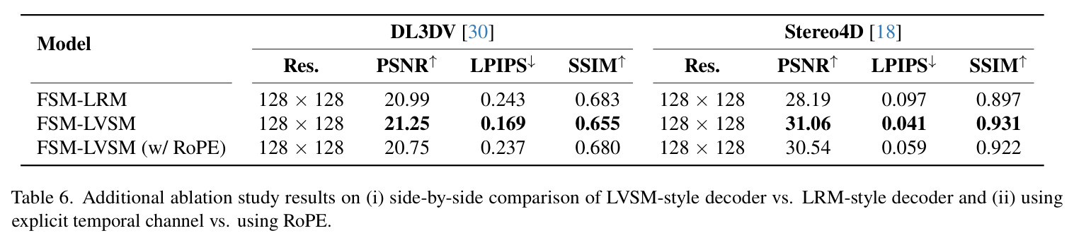
| 显式时间戳 vs RoPE(FSM-LVSM, 128×128) | PSNR / LPIPS / SSIM on DL3DV | 显式时间通道: 21.25 / 0.169 / 0.655 | RoPE: 20.75 / 0.237 / 0.680 | +0.50 dB PSNR,LPIPS 降低 28.7% |
局限与改进
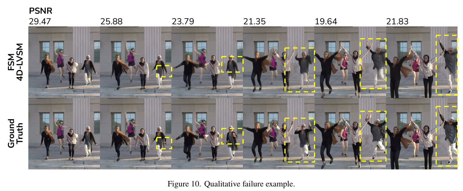
作者明确承认三点局限。第一,受限于可商用数据和算力,FSM 没有像 tttLVSM 那样在 540×960 上做长训练;当前 FSM 最高只在 256×256 上做 80K+10K 步训练,因此和 tttLVSM 540×960 的 26.90 dB 在分辨率对齐前不能直接比较。第二,FSM 假设相机 pose 已知,动态场景中的联合位姿估计并未处理——这是论文结论部分独立列出的一个开放问题。第三,仅靠渲染监督,模型仍会 '作弊' 走相机姿态插值捷径:在连续视角设定下,LaCET 虽明显好于 LaCT 但差距没有稀疏视角下那么大,说明没有显式几何监督时模型并不总能学到真正的 4D 表征。从失败案例(图 10)看,大视角/位姿外推时仍会出现 ghosting 和 stale 动作残留(PSNR 可低至 19.64)。
独立分析的弱点
从独立分析看,论文至少存在以下可改进点。其一,Fisher 估计的三种形式(EWC/MAS/SI)虽然都被尝试,但消融表中 streaming-EMA + MAS 的训练损失 (2.28) 高于 LaCT 单块 (1.80),说明弹性先验是 '以训练拟合换测试泛化',未来可以用更平滑的 importance surrogate(例如基于二阶曲率而非一阶梯度平方)来缩小训练损失。其二,4D Gaussian Splatting 版本 FSM-LRM 整体指标明显弱于 FSM-LVSM(DL3DV 上 PSNR 23.59 vs 26.69,Stereo4D 上 27.29 vs 32.16),作者把它归因于显式表征 '更难优化且更贵',但没有给出系统改进路径——一个直接的方向是为 FSM-LRM 设计更稳的 GS 参数化(多视角一致性 loss 或更短的 scale 范围)。其三,模型只在 256×256 训练,缺少对相机极端外推的鲁棒性(与高频细节),加一个 super-resolution / 多尺度一致性分支可能缓解。其四,测试时只允许 batch size = 1,因为 batched inference 会把多场景的更新平均掉,限制吞吐,未来可考虑 per-sample fast-weight buffer。
未来方向
作者在结论里给出三个明确方向:(1) 把 LaCET 真正扩展到数千帧长视频,做大数据+大模型+大分辨率的 scaling law;(2) 把联合相机位姿估计引入到 LaCET 框架,去除 'posed input' 这一前提;(3) 加入深度、光流、对应点等几何监督,使模型在 4D 表征上几何一致,而非只在新视角上像素一致。基于成果可延伸的方向包括:把 LaCET 当作通用快速权重 backbone 推广到视频生成、机器人策略学习等其它长序列场景;用更稳的 Fisher 估计(如 K-FAC 近似)替代一阶 EMA;以及在 4DGS head 端引入运动场分解,让前景/背景用不同 anchor 策略以更精细地利用弹性先验。
复现评估
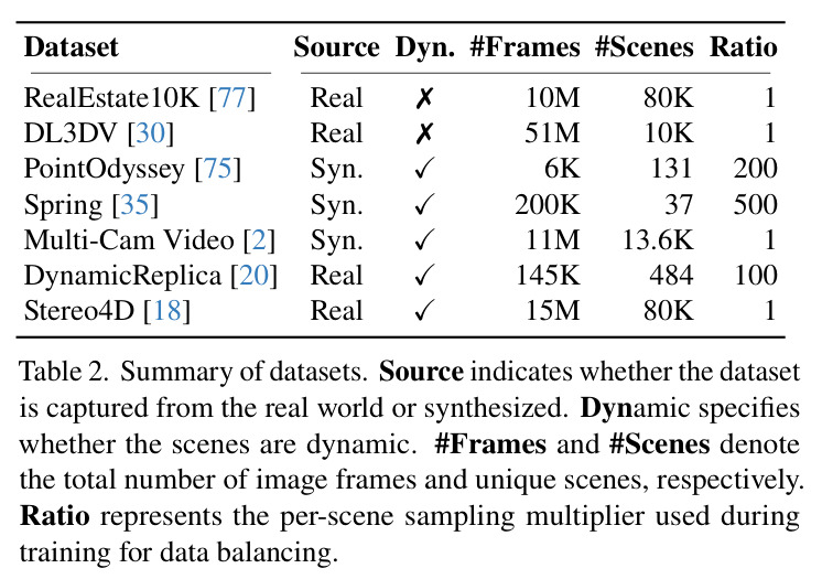
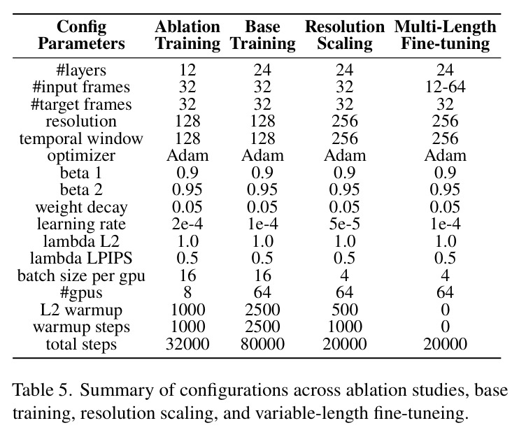
论文在 arXiv:2604.07350 公开,附带项目页 fast-spatial-memory.github.io。代码与权重未在正文声明开源链接,但附录 A.2 详细列出了 $\alpha_{ewc}=\beta_{ewc}=\lambda_{ewc}=0.5$、模型维度 768、SwiGLU hidden 1536、12 头 window attention (head dim 64)、QK-Norm、FFN 3072 等全部超参;附录 A.4 给出 '先 128×128 训 80K 步,再 256×256 微调 10K 步,64 张 H100' 的完整 recipe,复现门槛主要在算力(8×H100 起步做消融,64×H100 做完整预训练)。数据混合也已公开(Table 2),其中 4D 数据是 Stereo4D 主导,3D 静态数据是 DL3DV+RealEstate10K 主导。整体而言硬件依赖度高,但算法层细节充分,第三方在没有 64 张 H100 的情况下也可以复现 12 层消融版本。
论文图表