基于神经网络的分数梯度粒子方法求解Vlasov-Maxwell-Landau系统 A Neural Score-Based Particle Method for the Vlasov-Maxwell-Landau System
用神经网络替代kernel估计实现O(n)复杂度的等离子体碰撞模拟
前置知识
Vlasov-Maxwell-Landau系统
描述等离子体动力学的六维相空间偏微分方程组,包含Vlasov输运方程(描述粒子在自洽电磁场中的运动)和Landau碰撞算子(描述Coulomb碰撞)。这是一个多尺度、高维度的非线性系统,具有质量、动量和能量守恒性质,熵单调递减(H定理)。系统形式为$\partial_t f + v \cdot \nabla_x f + (E + v \times B) \cdot \nabla_v f = \nu Q[f,f]$,其中$f(t,x,v)$是分布函数,$Q$是Landau算子。
本文核心求解对象,理解这个系统的物理性质(守恒律、熵结构)才能理解作者如何设计保持这些性质的数值方法
Score函数
Score函数定义为$s(x,v) = \nabla_v \log f(x,v)$,即分布函数关于速度的对数梯度。Landau碰撞算子可以重写为以score函数驱动的输运方程:$Q[f,f] = \nabla_v \cdot \{f U(t,x,v)\}$,其中碰撞力$U$依赖于score函数的差异$s(x,v) - s(y,w)$。这个转换将碰撞问题从估计分布函数本身转换为估计score函数,使确定性格子方法成为可能。
本文方法的核心,作者用神经网络拟合这个函数,相比传统的KDE估计获得更好的精度和效率
Implicit Score Matching (ISM)
一种训练神经网络估计score函数的技术。原始目标是$\mathbb{E}_f[\|s_\theta - \nabla_v \log f\|^2]$,直接计算需要知道真实分布。通过分部积分消去真实score,得到等价的ISM损失:$L(\theta) = \mathbb{E}_f[\|s_\theta\|^2 + 2\nabla_v \cdot s_\theta]$。散度项用Hutchinson迹估计器计算:$\nabla_v \cdot s_\theta \approx z^\top \nabla_v s_\theta z$,其中$z$是Rademacher随机向量,只需一次前向自动微分。
本文SBTM方法的核心算法,使得能在粒子数据上以$O(n)$成本训练score网络,无需知道真实分布
Blob方法
一种基于核密度估计的score函数估计方法。公式为$s_{\text{KDE}}(x,v) = \nabla_v \log \sum_q w_q K_h(v-v_q) \psi_\eta(x-x_q)$,其中$K_h$是高斯核,$\psi_\eta$是空间localization核(如hat函数)。需要计算所有粒子对的核评估,复杂度$O(n^2)$。核带宽$h$的选择至关重要:太小导致噪声,太大导致过度平滑,尤其在低密度尾部区域容易产生系统性误差。
本文的baseline方法,理解其$O(n^2)$复杂度和带宽选择困难才能理解SBTM的优势所在
粒子网格法(PIC)
高维动力学模拟的主导方法。粒子在拉格朗日框架中推进(ODE方程$d x_p/dt = v_p$, $d v_p/dt = E + v_p \times B - \nu U^\eta$),而电磁场在空间网格上求解。通过deposit和插值操作耦合:粒子贡献电荷和电流密度到网格(用$\psi_\eta$核),网格求解Maxwell方程,场再插值回粒子位置。本文用hat函数(degree-1 B-spline)作为空间核,Yee差分格式离散化Maxwell方程。
本文采用的计算框架,SBTM作为drop-in replacement替换其中的score估计模块
研究动机
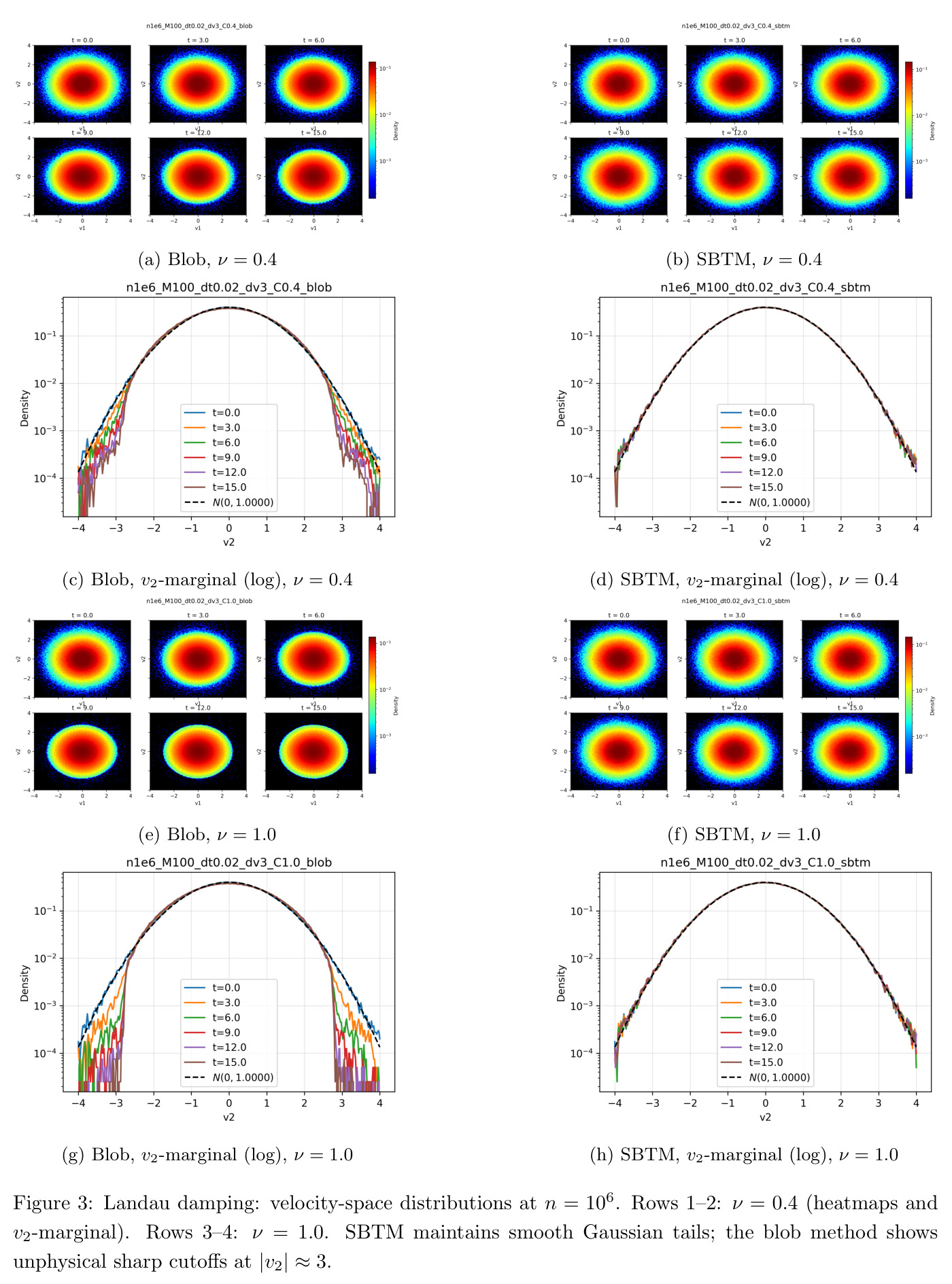
现有确定性格子方法[1]使用blob方法(基于核密度估计)来估计速度score函数,这带来了两个关键问题。首先,计算复杂度为$O(n^2)$,因为需要在每个空间网格内计算所有粒子对的核评估,这在大规模模拟($n = 10^6$粒子级别)中成为瓶颈。其次,核带宽的选择非常困难:带宽太大会过度平滑分布,丢失低密度尾部的信息;带宽太小会导致噪声累积,尤其在稀疏粒子区域。这种score估计误差在长时间弛豫到Maxwellian平衡态时会累积成系统性伪影,导致物理上不正确的结果。例如在Landau阻尼和Weibel不稳定性测试中,blob方法产生不自然的尖锐截止而非光滑的高斯尾部。
本文的目标是本文的目标是将Score-Based Transport Modeling (SBTM)应用到完整的Vlasov-Maxwell-Landau系统中,替代blob方法进行score函数估计。具体目标包括:(1) 实现线性复杂度$O(n)$的score估计,大幅提升大规模模拟的效率;(2) 改善低密度区域的score估计精度,使得系统能够正确弛豫到Maxwellian平衡态;(3) 证明离散化碰撞算子的守恒性质(动量、动能、熵耗散);(4) 理论上刻画VML和VPL系统的全局稳态,为数值验证提供ground truth。
与已有工作不同的是,本文的独特切入点在于将原本用于空间齐次Landau方程的SBTM[20]扩展到空间非齐次且与电磁场耦合的完整VML系统。这带来了新的技术挑战:需要空间localization(用hat核$\psi_\eta$),需要耦合Maxwell场求解器,需要用单个网络处理不同空间网格中截然不同的速度分布。作者通过在t=0预训练网络于初始条件的解析score,然后每个时间步执行K次ISM梯度步来在线适应演化中的分布,同时保持物理一致性。这种'on-the-fly'训练策略是相对于离线预训练方法的关键区别。
核心方法
方法整体思路是将Landau碰撞算子重写为以score函数驱动的输运方程,然后用神经网络在线学习这个score函数。直觉上,score函数$\nabla_v \log f$告诉我们在速度空间哪个方向概率密度增长最快,碰撞力正是依赖于不同位置的score差异。技术路线上,作者保持原有的PIC框架(粒子ODE推进 + 场网格求解),只替换score估计模块:blob方法的KDE计算被替换为神经网络的ISM训练。空间上用hat核$\eta$进行localization,每个粒子只与同网格或相邻网格的粒子碰撞。神经网络是两层MLP,softsign激活,隐藏层维度256或512。每个时间步,网络在当前粒子数据上执行K次AdamW梯度步,损失函数是particle average的ISM损失,复杂度$O(n)$。
核心创新点是用隐式score matching训练的神经网络替代传统的核密度估计来估计score函数。与blob方法的本质区别在于:blob方法直接用核平滑粒子分布然后求导,这是非参数估计且需要$O(n^2)$计算;而SBTM用参数化函数(神经网络)拟合score,通过ISM损失(particle数据上可计算)在线学习,复杂度$O(n)$。另一个关键区别是泛化能力:神经网络能从观测区域学习到score函数的整体结构,从而在低密度尾部给出合理的推断,而KDE在这些区域受限于数据稀缺。这种能力使得SBTM能够正确捕捉Maxwellian平衡态的线性score($s \propto -v$),而blob方法产生噪声和不连续的估计。
方法步骤详情
方法步骤的完整描述如下。输入:$n$个粒子$\{(x_p, v_p, w_p)\}_{p=1}^n$,网格场$\{E_j, B_j\}_{j=1}^M$,时间步$\Delta t$,碰撞频率$\nu$,ISM步数$K$,空间核$\psi_\eta$,碰撞核$A(z)=|z|^{\gamma+2}\Pi(z)$。输出:更新后的粒子和场。步骤:(1) 预训练:在t=0用初始条件的解析score预训练网络$s_\theta$。(2) 网格到粒子:$E_p = \eta \sum_j \psi_\eta(x_p-x_j) E_j$,$B_p = \eta \sum_j \psi_\eta(x_p-x_j) B_j$。(3) Lorentz推进:$v_p \leftarrow v_p + \Delta t (E_p + v_p \times B_p)$。(4) 位置更新:$x_p \leftarrow x_p + \Delta t v_{1,p}$(模L周期边界)。(5) 粒子到网格:$\rho_j = \sum_p w_p \psi_\eta(x_j-x_p)$,$J_{i,j} = \sum_p w_p v_{i,p} \psi_\eta(x_j-x_p)$。(6) 场更新:用Yee格式离散化Maxwell方程,$E_{1,j} \leftarrow E_{1,j} - \Delta t J_{1,j}$,$E_{2,j} \leftarrow E_{2,j} - \Delta t [(B_{3,j+1}-B_{3,j-1})/(2\Delta x) + J_{2,j}]$,$B_{3,j} \leftarrow B_{3,j} - \Delta t (E_{2,j+1}-E_{2,j-1})/(2\Delta x)$。(7) ISM训练:重复K次:抽取Rademacher随机向量$z \sim \text{Rademacher}(\pm 1)^{d_v}$,计算梯度步$\theta \leftarrow \theta - \alpha \nabla_\theta [\sum_p w_p (\|s_\theta(x_p,v_p)\|^2 + 2z^\top(\nabla_v s_\theta(x_p,v_p))z)]$,学习率$\alpha = 2 \times 10^{-4}$。(8) 碰撞更新:$v_p \leftarrow v_p - \Delta t \nu \sum_q w_q \psi_\eta(x_p-x_q) A(v_p-v_q)[s_\theta(x_p,v_p) - s_\theta(x_q,v_q)]$。(9) 时间推进:$t \leftarrow t + \Delta t$,重复直到$t = t_{final}$。
技术新颖性
技术新颖性体现在多个方面:(1) 首次将SBTM应用到完整的Vlasov-Maxwell-Landau系统,之前工作[20]仅限于空间齐次Landau方程。这需要处理空间非齐次性(localization核$\psi_\eta$)和电磁场耦合(Maxwell求解器)。(2) 理论贡献:证明了离散化碰撞算子对任意score近似都保持动量和动能守恒,并耗散估计熵(Theorem 2.3)。还首次完整刻画了VML和VPL系统的全局稳态(Theorems 2.1和2.2),提供了数值验证的理论基准,Theorem 2.1还在Lean 4中形式化验证[19]。(3) 实现创新:用'on-the-fly'训练策略,每个时间步执行K次梯度步,网络持续适应演化中的分布。初始预训练在解析score上加速收敛。(4) 效率优势:将score估计从$O(n^2)$降到$O(n)$,在大规模模拟中带来显著速度和内存提升。实验显示1.57×速度提升,2-4×内存降低。
实验结果
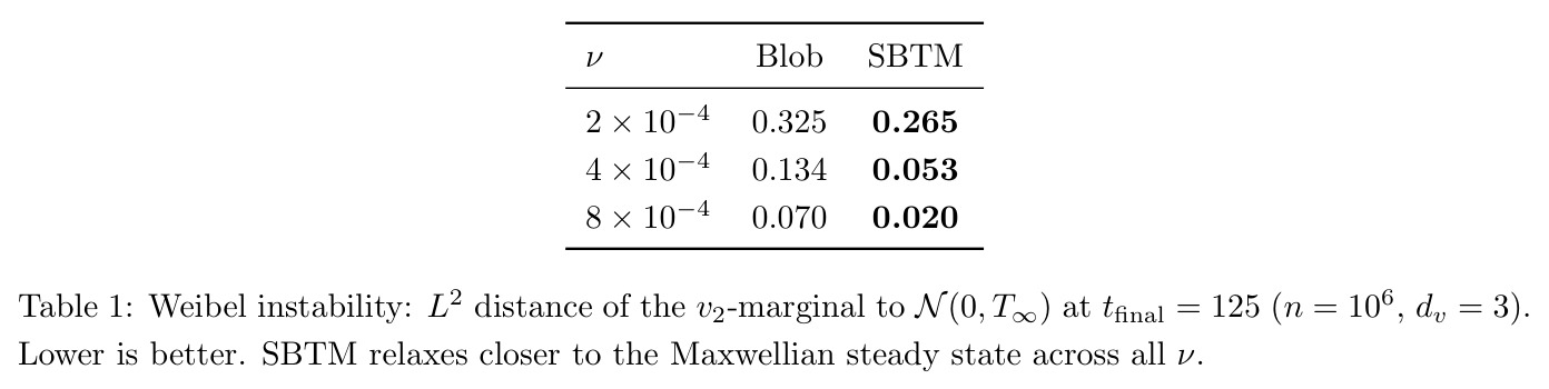
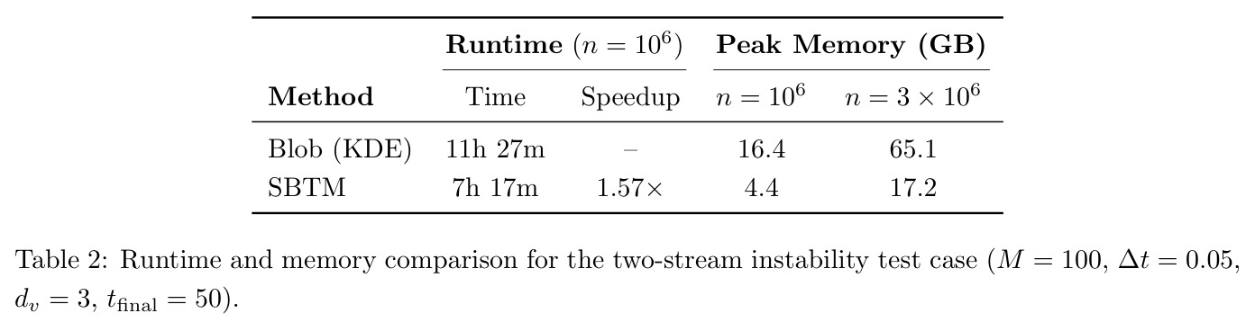
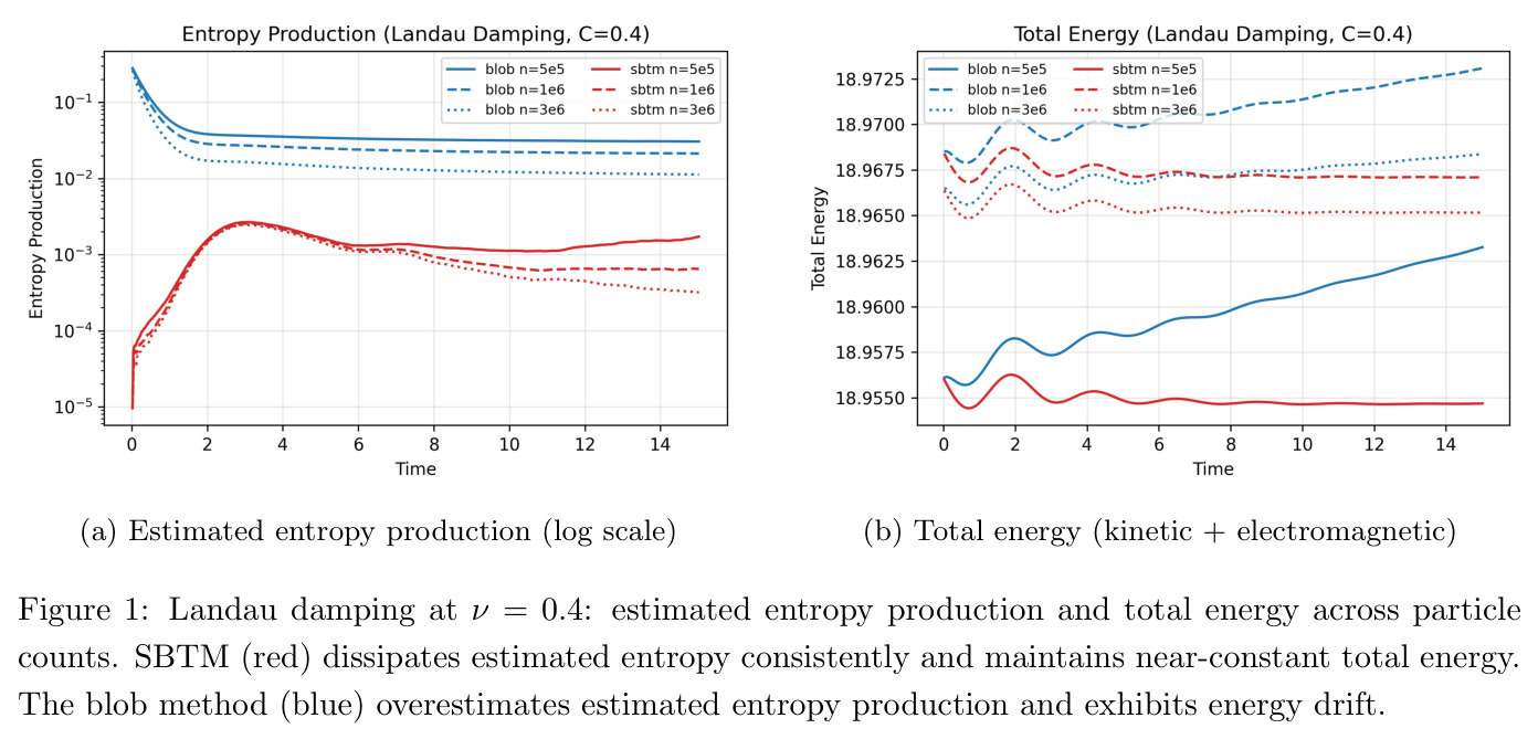
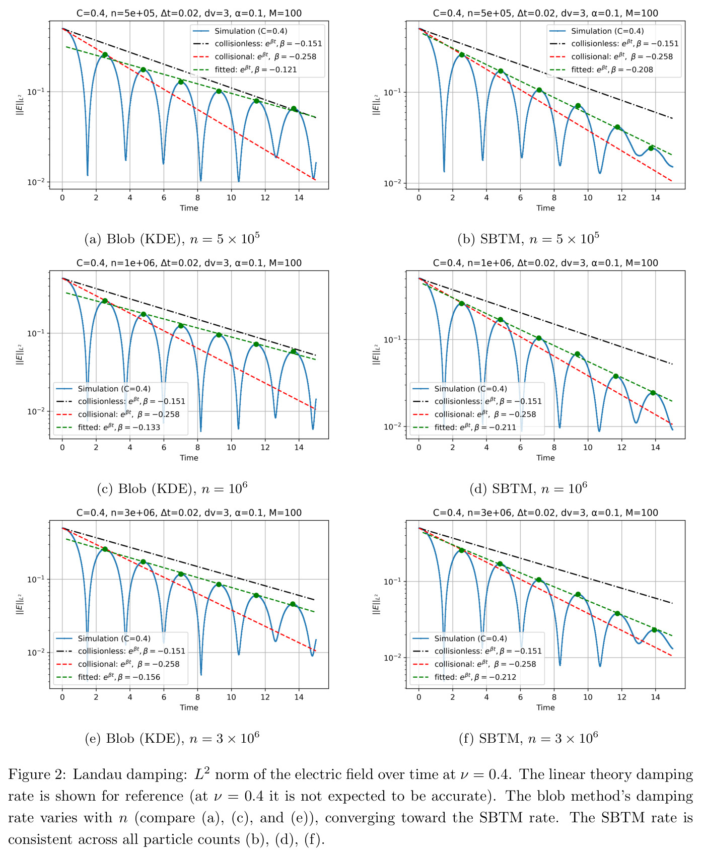
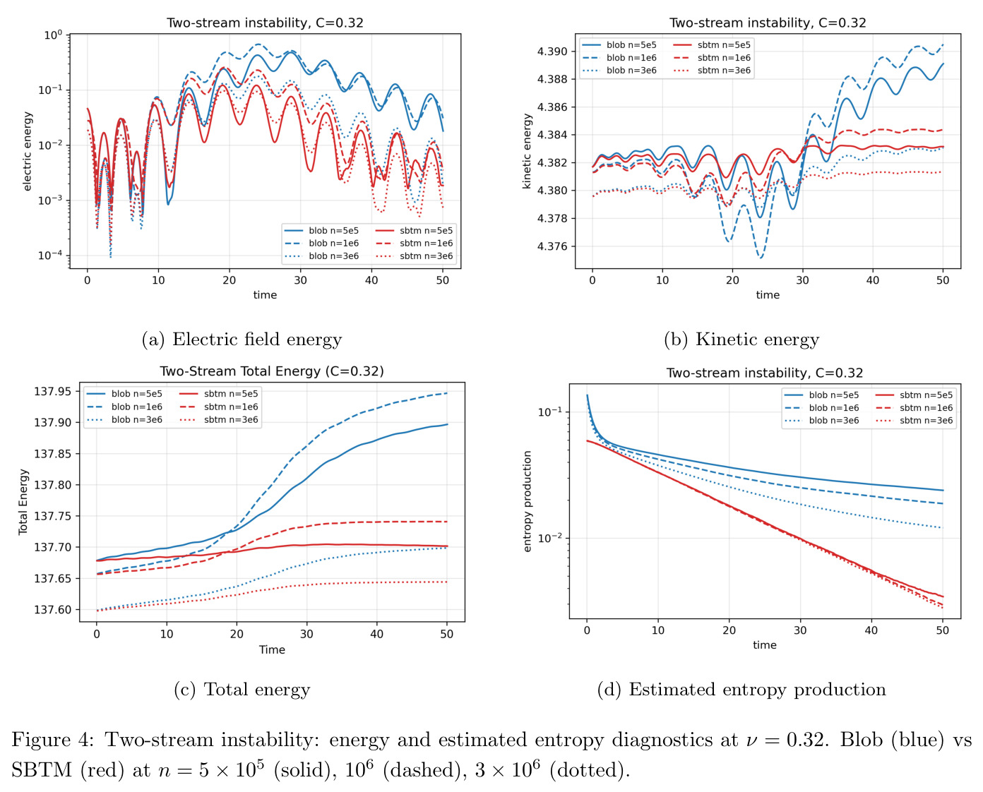
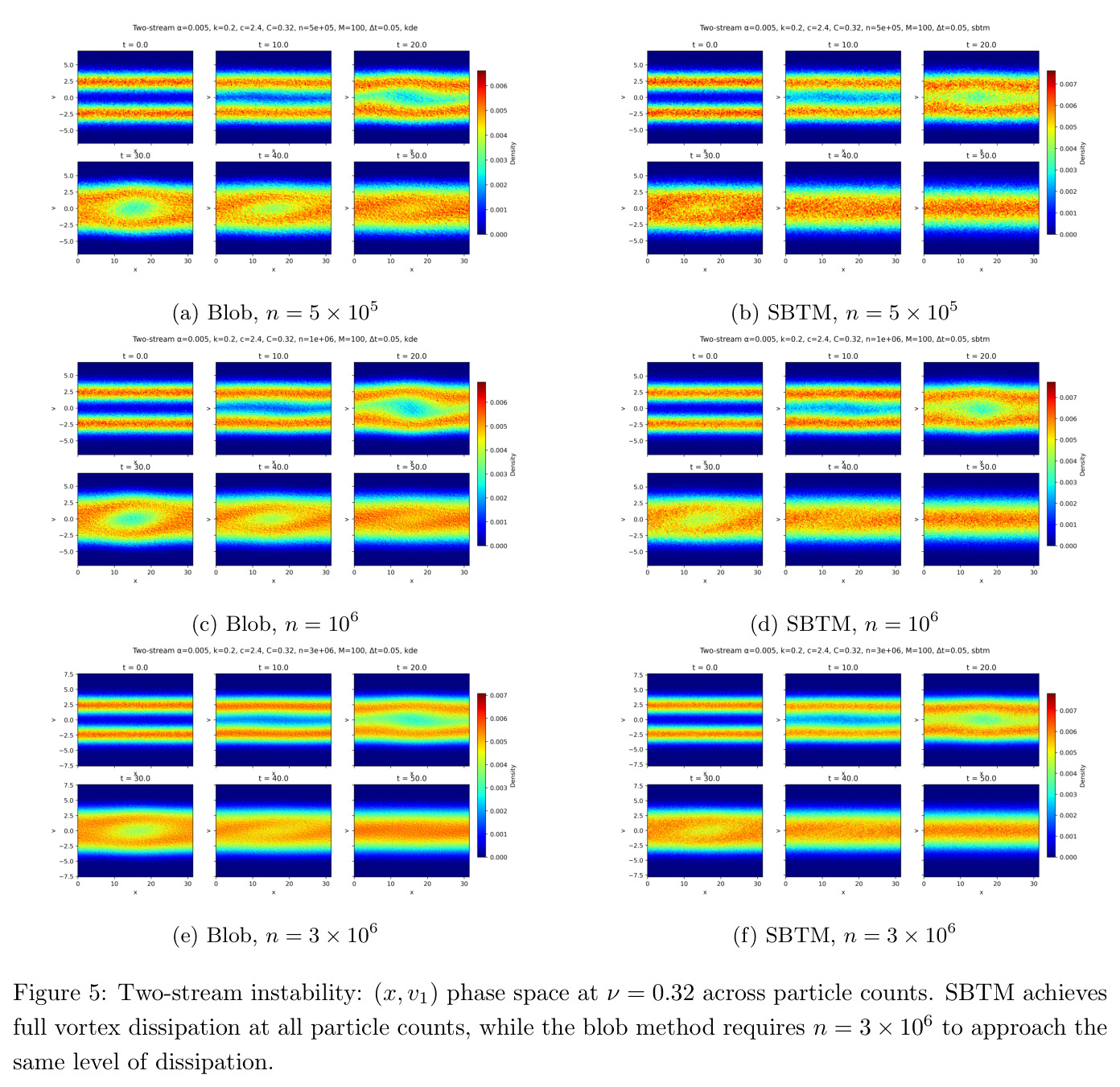
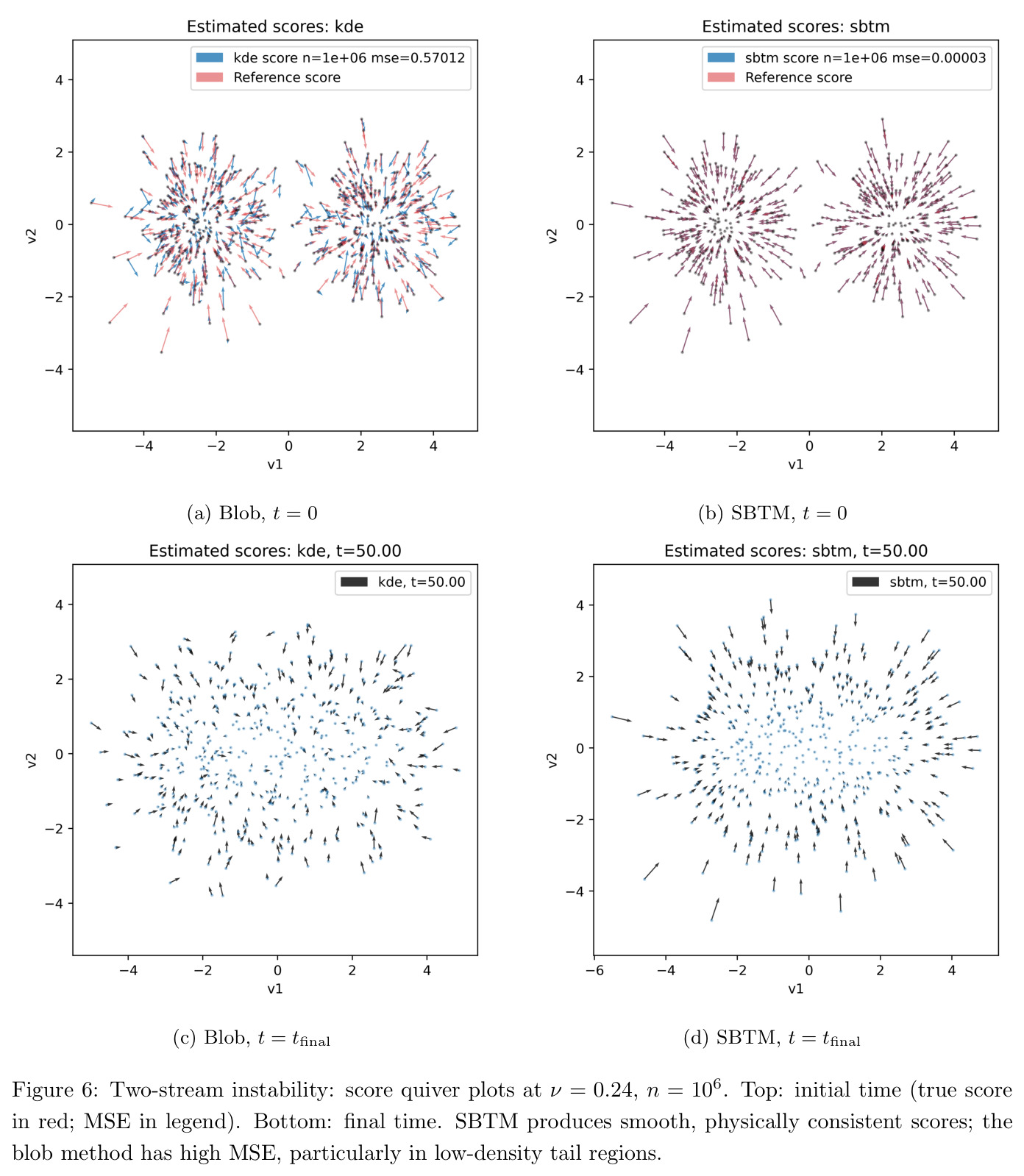
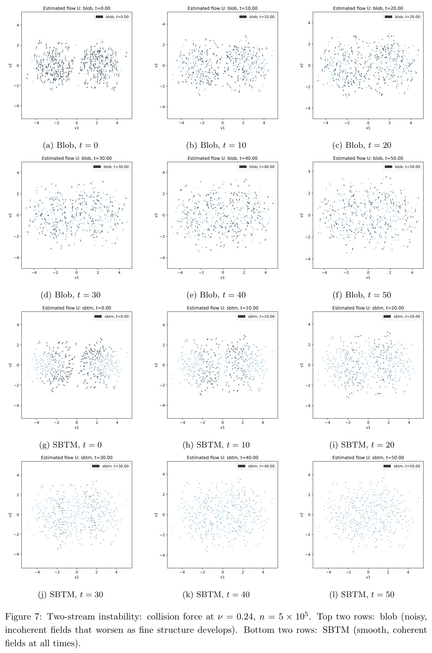
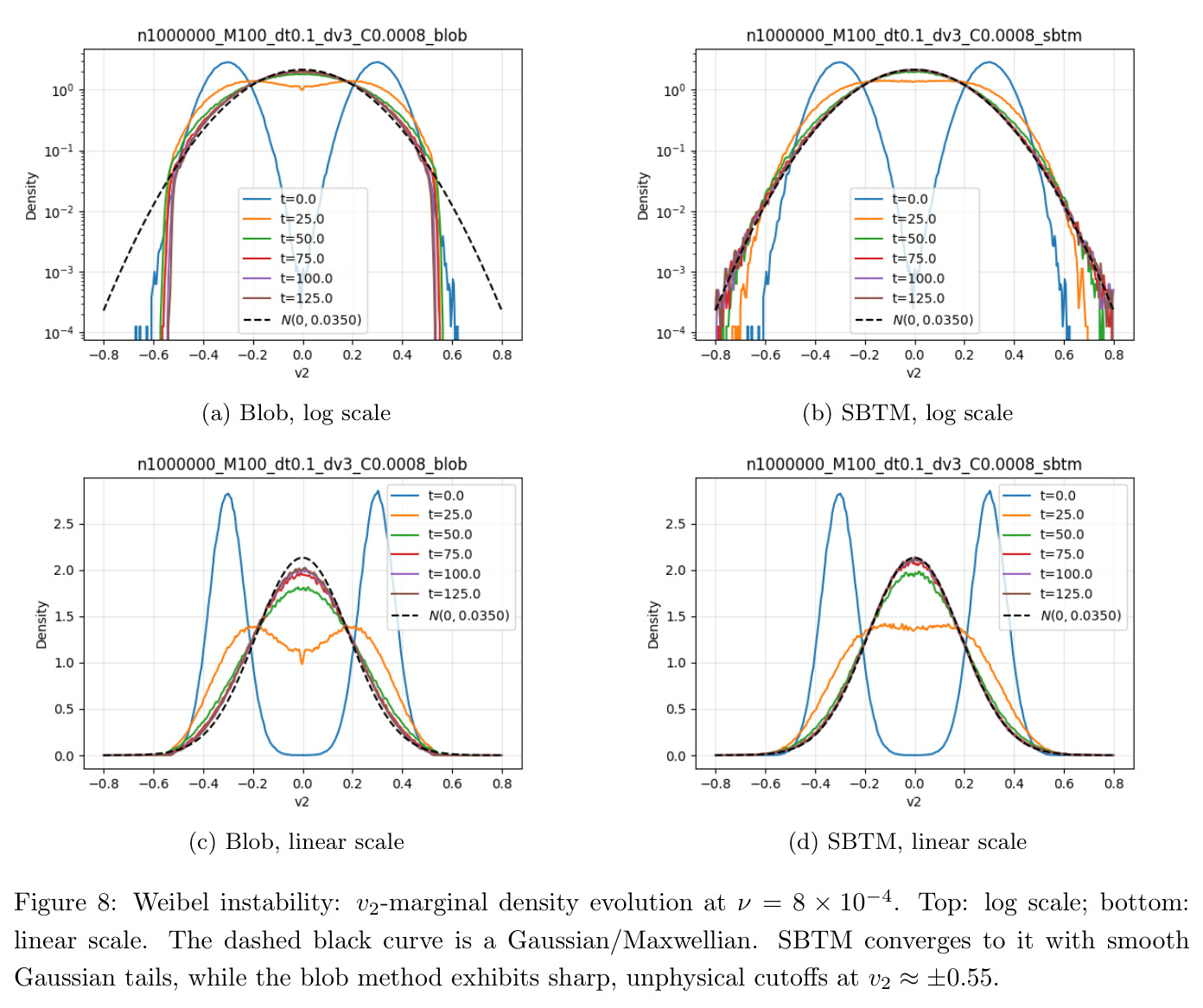
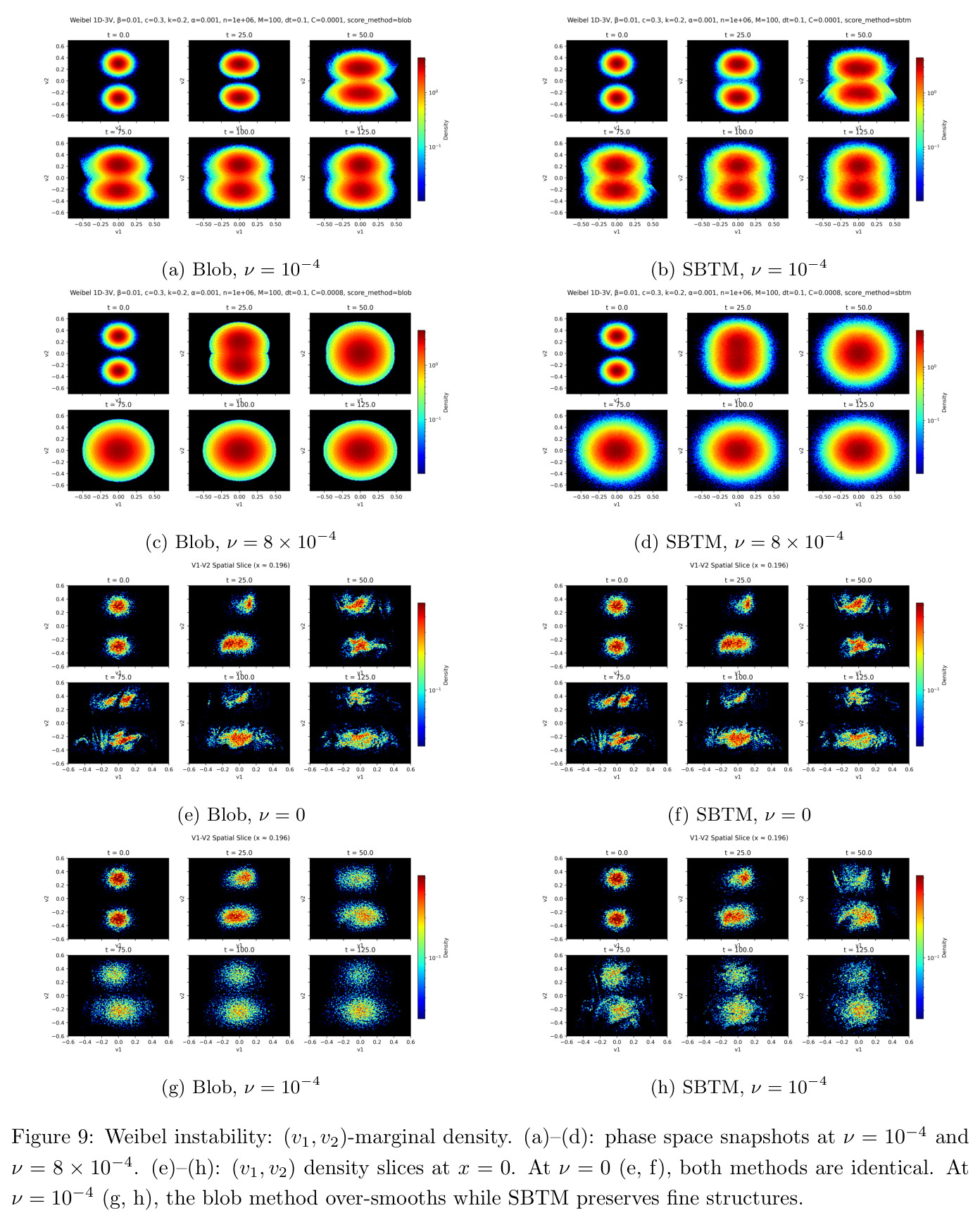
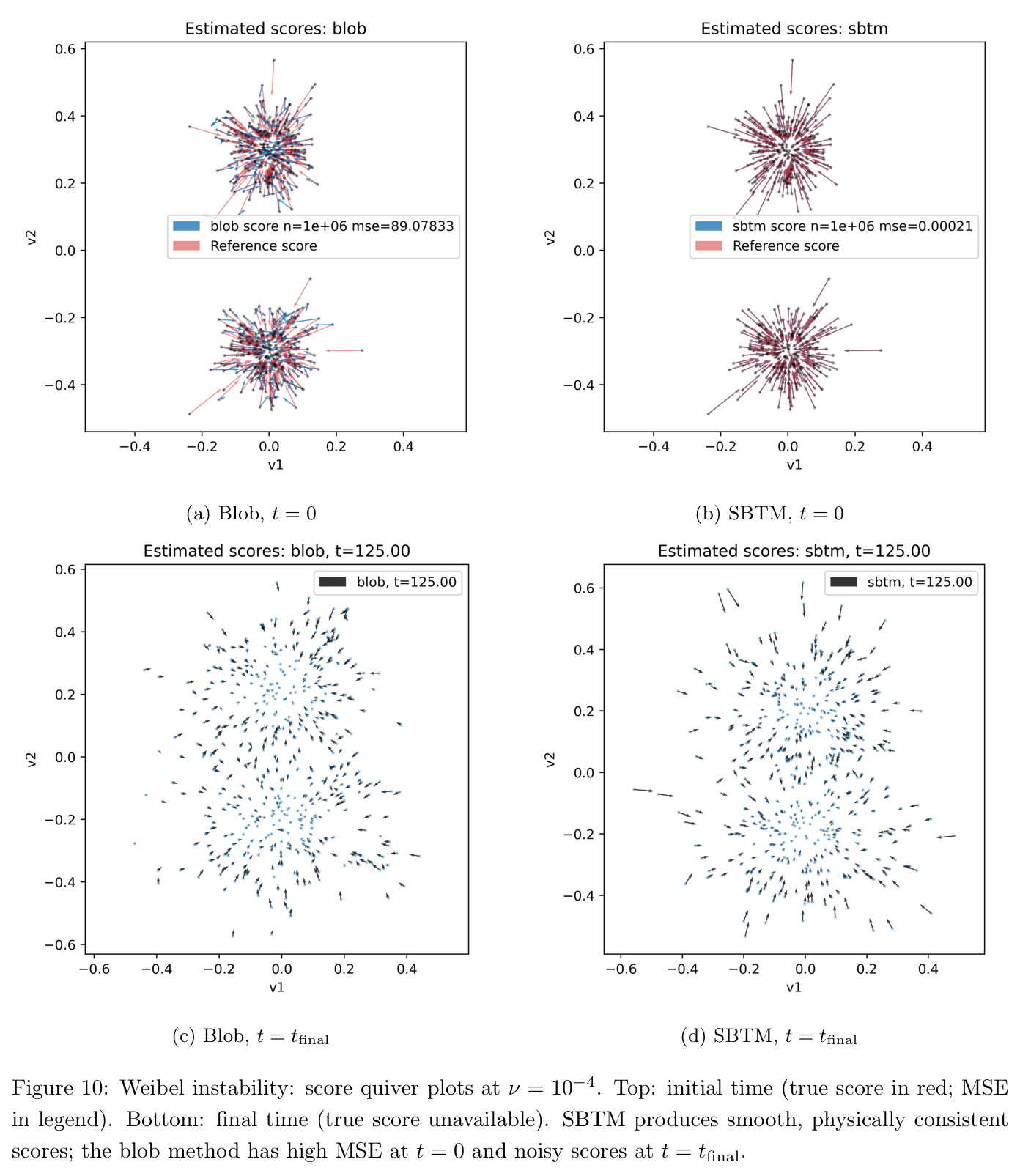
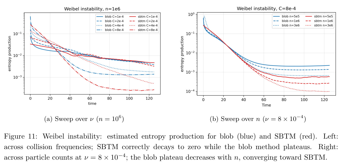
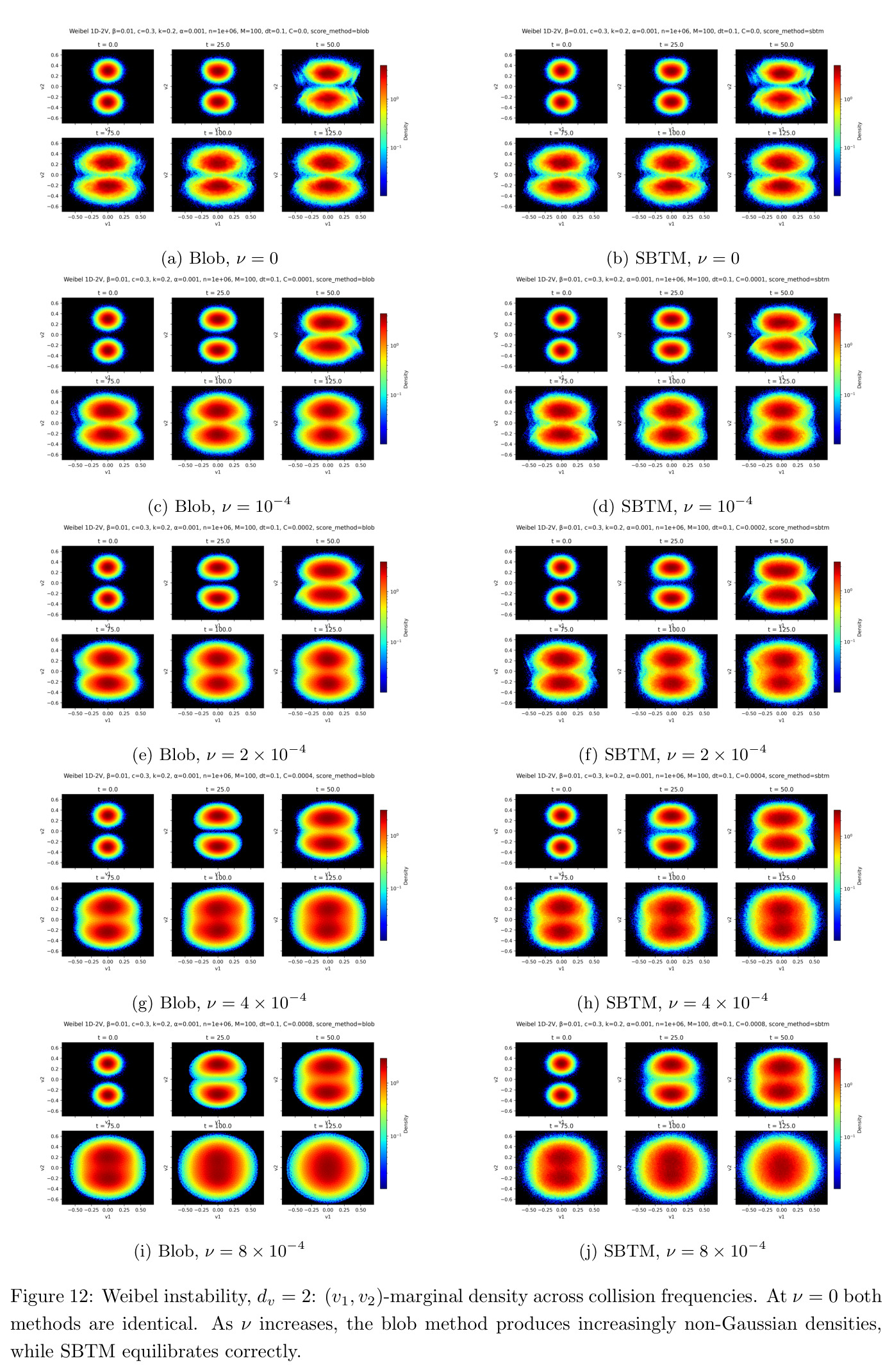
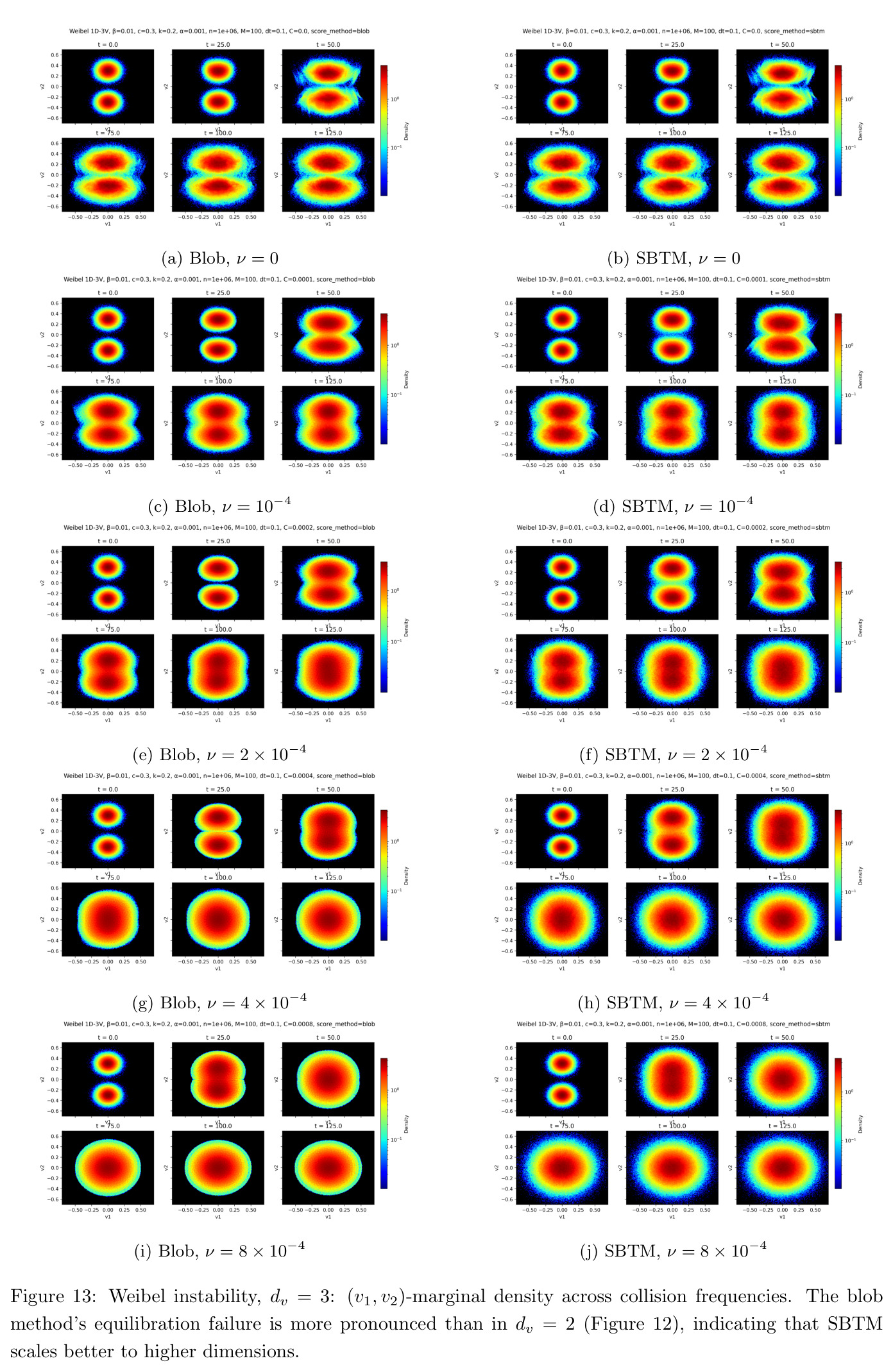
核心发现来自三个基准测试的详细分析。Landau阻尼($n \in \{5 \times 10^5, 10^6, 3 \times 10^6\}$,$\nu=0.4$):SBTM在所有粒子数下产生一致的估计熵产生曲线,正确衰减到零(符合平衡态预期);blob方法在低n时严重高估,即使在$n=3 \times 10^6$仍偏离SBTM曲线。电场$L^2$衰减率:SBTM率在所有n下保持一致,blob率随n变化,高n时才趋近SBTM率,表明SBTM收敛更快。速度分布:SBTM保持光滑高斯尾部,blob方法在$|v_2| \approx 3$处产生不自然的尖锐截止。Two-Stream不稳定性($c=2.4$,$\nu=0.32$):SBTM在所有n下实现完整的相空间涡旋耗散(t=50),blob方法需要$n=3 \times 10^6$才能接近。分数估计:t=0时SBTM的MSE远低于blob(解析score已知);t=50时SBTM分数光滑且物理一致(向量指向原点,幅值随距离增加),blob分数在低密度尾部嘈杂。碰撞力场:SBTM保持初始条件的对称性($v_1 \to -v_1$和$v_2 \to -v_2$),并在t=50消失;blob方法破坏对称性且t=50仍存在。Weibel不稳定性(各向异性双Maxwellian,$c=0.3$,$\beta=0.01$,$n=10^6$,$\nu \in \{10^{-4}, 2 \times 10^{-4}, 4 \times 10^{-4}, 8 \times 10^{-4}\}$):SBTM在所有$\nu$下收敛到预期Maxwellian $N(0, T_\infty=0.035)$且尾部光滑;blob方法在$v_2 \approx \pm 0.55$处产生尖锐截止。$v_2$-边际到Maxwellian的$L^2$距离:在$\nu=8 \times 10^{-4}$,blob为0.070,SBTM为0.020(3.5×更近);$\nu=2 \times 10^{-4}$,blob为0.325,SBTM为0.265(1.2×更近)。估计熵产生:SBTM在所有$\nu$下正确衰减到零,高$\nu$衰减更快;blob方法在非零值平台(尾部score误差持续)。固定$\nu=8 \times 10^{-4}$,blob平台随n增加下降,趋近SBTM。计算效率:Two-Stream测试($n=10^6$,$t_{final}=50$,$M=100$,$\Delta t=0.05$,$d_v=3$):SBTM运行时间7小时17分钟,blob 11小时27分钟(1.57×加速);峰值内存:SBTM 4.4GB,blob 16.4GB(3.7×降低)。$n=3 \times 10^6$时:SBTM 17.2GB,blob 65.1GB(3.8×降低)。
查看结构化数据
| 任务 | 指标 | 本文 | 基线 | 提升 |
|---|---|---|---|---|
| Landau阻尼熵产生精度 | 估计熵产生在长时间衰减至零 | 所有粒子数($5\times10^5$-$3\times10^6$)均正确衰减至零 | 低粒子数时严重高估,$3\times10^6$时仍偏离正确值 | 定性提升:正确的物理行为 vs 系统性误差 |
| Landau阻尼速度分布 | 低密度尾部光滑度 | 光滑高斯尾部,无人工截止 | 在$|v_2| \approx 3$处尖锐截止 | 定性提升:物理合理 vs 人工伪影 |
| Two-Stream涡旋耗散 | t=50时相空间涡旋完全耗散所需粒子数 | 所有粒子数($5\times10^5$-$3\times10^6$)均实现 | 需要$3\times10^6$粒子 | 6×收敛加速(从$3\times10^6$到$5\times10^5$) |
| Two-Stream分数估计(t=0) | 相对于解析score的MSE | 低MSE | 高MSE(约为SBTM的数倍) | 数倍精度提升(具体数值未给出) |
| Weibel不稳定性平衡态距离 | $v_2$-边际到Maxwellian的$L^2$距离 | 0.020 ($\nu=8\times10^{-4}$) | 0.070 ($\nu=8\times10^{-4}$) | 3.5×更接近真实平衡态 |
| Weibel不稳定性平衡态距离 | $v_2$-边际到Maxwellian的$L^2$距离 | 0.265 ($\nu=2\times10^{-4}$) | 0.325 ($\nu=2\times10^{-4}$) | 1.2×更接近真实平衡态 |
| Two-Stream运行时间 | Wall-clock时间 ($n=10^6$) | 7小时17分钟 | 11小时27分钟 | 1.57×加速 |
| Two-Stream峰值内存 | GPU内存占用 ($n=10^6$) | 4.4GB | 16.4GB | 3.7×降低 |
| Two-Stream峰值内存 | GPU内存占用 ($n=3\times10^6$) | 17.2GB | 65.1GB | 3.8×降低 |
局限与改进
局限性分析包括作者承认的和观察到的。作者明确指出:(1) 时间积分采用前向欧拉格式,不能在完全离散水平保持能量守恒(尽管半离散水平守恒)。作者提到可以采用[33]的能量守恒显式格式,但代价是每步需要2-3次碰撞算子评估。(2) 所有实验限制在$1D_x$空间设置,单电子种类,不可动中性离子背景。实际应用需要扩展到多维空间和多组分等离子体。此外,我观察到:(3) 每个时间步需要K=100次ISM梯度步,虽然每次是$O(n)$,但总计算成本仍可观。减少K或使用更高效优化器是潜在优化方向。(4) 神经网络架构是简单的两层MLP,未探索更复杂架构如Transformer。虽然作者提到DiScoFormer[21]作为无重训练的替代,但'on-the-fly'训练对处理演化中的分布可能是必要的。(5) 实验的碰撞频率范围有限($\nu \in [10^{-4}, 1.0]$),更高碰撞频率下SBTM的鲁棒性未充分验证。(6) 网格大小M=100固定,空间分辨率对score估计质量的影响未系统研究。高分辨率可能需要更精细的空间localization或多个独立网络。
独立分析的弱点
独立分析的弱点包括:(1) 训练开销:每个时间步100次ISM梯度步,虽然单次是$O(n)$,但累积成本显著。改进方向:使用自适应K(熵产生变化大时增加,平稳时减少);探索更高效的优化器如L-BFGS;利用JAX的just-in-time编译和批处理优化。(2) 网络容量限制:简单MLP可能难以捕捉复杂的多峰分布,尤其在强非平衡态。改进方向:使用更深层或条件化网络;引入attention机制捕捉长程相关性;探索条件归一化流作为score函数模型。(3) 空间localization粗糙:单hat核将空间划分为网格,忽略了跨网格的长程碰撞。改进方向:使用多尺度核或可学习的空间权重;为不同空间区域训练专门的网络;探索图神经网络处理空间依赖。(4) 缺乏不确定性量化:神经网络输出确定性score,无法表达估计置信度。改进方向:贝叶斯神经网络;集成方法;输出方差估计。(5) 泛化到更高维度:虽然实验显示$d_v=3$表现良好,但$d_v > 3$的性能未验证。改进方向:设计专门针对高维score估计的网络架构;探索降维技术或factorized score表示。(6) 碰撞频率依赖性:不同$\nu$可能需要不同的学习率或网络超参数。改进方向:自适应超参数调度;将$\nu$作为网络输入条件。
未来方向
未来研究方向包括作者提出的和基于成果可延伸的。作者明确提到:(1) 采用能量守恒显式时间积分格式[33],改进完全离散水平的守恒性质。(2) 扩展到多空间维度($2D_x$、$3D_x$)和多组分等离子体(电子+多离子种类)。(3) 应用到更实际的等离子体物理问题,如托卡马克边缘等离子体、激光-等离子体相互作用等。基于成果可延伸的方向包括:(4) 探索替代训练策略:离线预训练+在线微调(减少每步梯度步数);元学习预训练以快速适应不同初始条件;连续学习防止 catastrophic forgetting。(5) 与其他碰撞算子结合:Fokker-Planck碰撞、库仑对数修正后的碰撞算子;研究SBTM对非标准碰撞核的适应性。(6) 不确定性量化和鲁棒性:集成SBTM;贝叶斯神经网络估计score不确定性;针对极端参数(极高$\nu$、极低密度)的鲁棒性分析。(7) 与传统方法混合:高频区域用SBTM,低频/平衡态附近用blob方法节省计算;基于局部误差指标的adaptive方法选择。(8) 物理约束学习:将守恒律作为硬约束加入网络设计;探索symplectic或H-结构保持的神经网络架构。(9) 硬件加速和优化:针对GPU和TPU的专门kernel优化;分布式训练支持更大规模模拟;量化和剪枝减少内存占用。(10) 理论扩展:SBTM收敛性的严格理论分析(目前仅有齐次情况[18]);误差传播分析;不同初始条件下稳态的唯一性和稳定性证明。
复现评估
复现评估:代码开源在GitHub (https://github.com/Vilin97/Vlasov-Landau-SBTM),使用JAX实现双精度计算。所有实验在华盛顿大学Hyak和Tillicum集群的NVIDIA L40S和H200 GPU上运行。Three-benchmark的详细参数在Section 3.1-3.4给出,包括网格数M、时间步$\Delta t$、粒子数n、碰撞频率$\nu$、ISM步数K、神经网络隐藏维度等。Landau阻尼:$L=2\pi/k$,$k=0.5$,$\alpha=0.1$,$d_v=3$,$M=100$,$\Delta t=0.02$,$\nu=0.4$,$t_{final}=15$,$K=100$,$n \in \{5 \times 10^5, 10^6, 3 \times 10^6\}$,隐藏层256。Two-Stream:$c=2.4$,$k=1/5$,$\alpha=1/200$,$d_v=3$,$M=100$,$\Delta t=0.05$,$\nu=0.32$,$t_{final}=50$,$K=100$,$n \in \{5 \times 10^5, 10^6, 3 \times 10^6\}$,隐藏层256。Weibel:$c=0.3$,$\beta=0.01$,$\alpha_B=10^{-3}$,$k=1/5$,$L=10\pi$,$d_v=3$,$M=100$,$\Delta t=0.1$,$n=10^6$,$t_{final}=125$,$K=100$,$\nu \in \{10^{-4}, 2 \times 10^{-4}, 4 \times 10^{-4}, 8 \times 10^{-4}\}$,隐藏层512。所有实验使用等权粒子$w_p = L/n$。代码依赖JAX、Flax (JAX的神经网络库)、Optax (优化器)。难度评估:中等-偏难。需要JAX编程经验,理解自动微分和粒子网格方法。计算资源要求高(高内存GPU),但论文给出的详细参数和开源代码使得复现可行。主要挑战可能是长时间运行(实验需要7-11小时),但可以使用较小的n或较短的$t_{final}$进行初步验证。
论文图表