从连续参数预测整数 Predicting integers from continuous parameters
系统比较并提出三种离散整数分布,用于神经网络直接输出整数值。
前置知识
概率质量函数与概率密度函数
离散随机变量用概率质量函数(PMF)$p(x)$ 直接给出 $P(X=x)$,所有点加起来等于 1;连续随机变量用概率密度函数(PDF)$f(x)$,积分等于 1,单点 $f(x)$ 本身没有概率意义。离散情形的负对数概率 $-\log p(x)$ 自然以 bit 为单位,而连续情形的负对数概率密度不具单位、不变量纲、且依赖变量选择。
本文反复利用这一区别:作者主张把整数标签用真正的离散分布建模,是为了得到物理意义明确的 bit 量纲损失,从而能与其它离散输出(如分类输出)相加比较。
反向传播与梯度下降对参数连续性的要求
PyTorch 等框架要求计算图上每个节点对参数可微。离散参数(如整数 $\mu$)没有局部梯度信息,因此用作神经网络输出分布的参数时必须是连续的,例如 $\mu \in \mathbb{R}$。本文的 Dalap/Danorm/Bitwise 都遵循这一原则:$\mu$ 和 $\gamma$ 都是连续标量。
这正是本文核心问题域——既要让样本空间(整数)保持离散,又让分布参数连续可微,是耦合两条性质的关键技术约束。
离散化连续分布 vs. 离散类比分布
「离散化」是先在实数域采样连续分布(如正态、拉普拉斯),再用舍入把实数压到最近整数;「离散类比」则直接构造一个定义在整数上的 PMF,使其形状特征(如尾部的指数衰减)保留连续版的关键属性。Dalap 与 Danorm 属于后者;Dlaplace 与 Dnormal 属于前者。
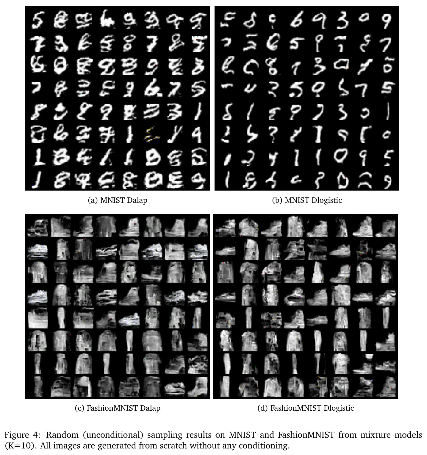
本文用实验证明:当用相同骨干网络时,离散类比(Dalap)在图像生成上能胜过 PixelCNN++ 的离散化 logistic(Dlogistic),说明「保留序数结构的真正离散」是重要设计选择。
Bits Per Dimension(BPD)与压缩视角的损失
对于 $N$ 维数据,用分布 $p$ 编码的期望 bit 数是 $\mathbb{E}[-\log_2 p(x)]$,除以维度数即 BPD。BPD 直接衡量「该分布给数据多少 bit」,等价于无损压缩码长。当多种分布都能产生合理样本时,BPD 提供一个跨模型可比的客观度量。
本文的图像实验几乎完全以 BPD 作为主要评估指标,作者也明确把「多种输出分布能用同一单位比较」作为离散分布的重要卖点。
研究动机
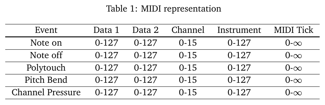
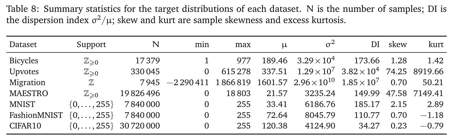
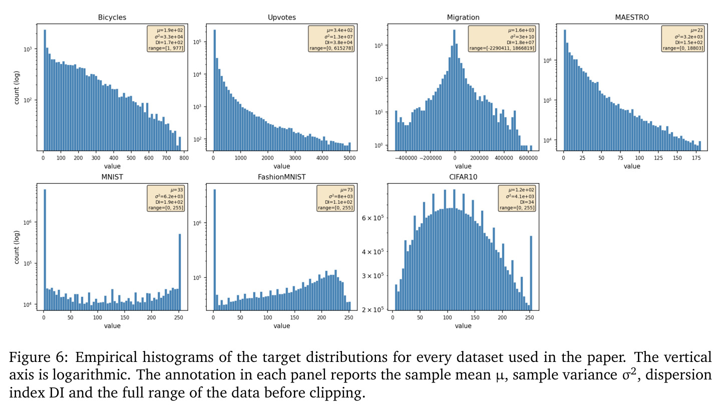
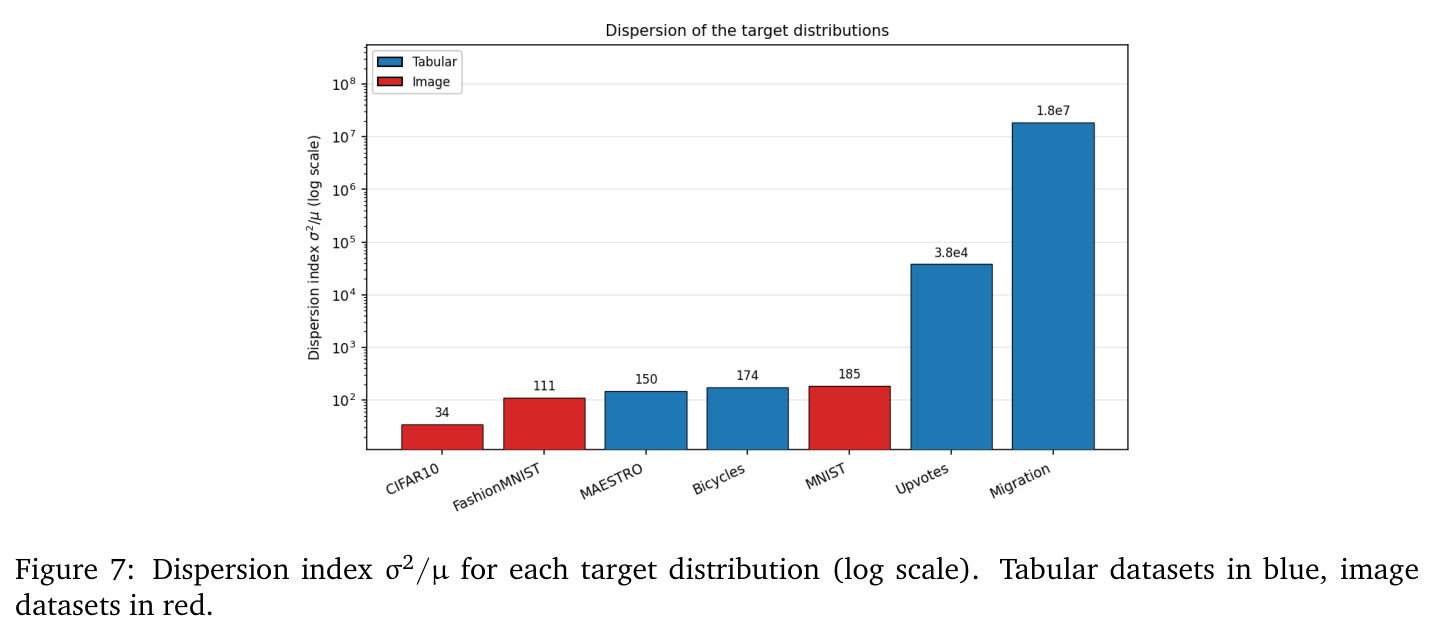
现实中有大量回归任务的标签天然是整数——比如社交媒体帖子的点赞数(Upvotes 数据集均值 337,峰度 8919,DI=3.82×10⁴,呈极端右偏)、公共自行车站可用车辆数(Bicycles DI=173.66)、国家间净迁徙人数(Migration 含正负值,方差 2.96×10¹⁰,DI=1.85×10⁷)、RGB 像素值(0–255 的固定区间)、MIDI 音符间隔 ticks。工业界普遍做法是「连续松弛」(continuous relaxation):用 MSE 等连续损失训练,推理时四舍五入到最近整数。这种做法的问题有三:第一,损失单位不可解释——连续 log-density 不以 bit 为单位、且依赖变量选择(Cover 1999 定理 8.6.4);第二,多任务合成损失时无法自然平衡——例如把油门推力(连续)和摇杆方向(离散分类)的损失相加,必须人为调权重;第三,对于像素这类数据,连续松弛在 Loaiza-Ganem & Cunningham (2019)、Rybkin et al. (2021) 等文献中已被证明显著劣于真正的离散建模。
本文的目标是本文目标是在「样本空间是离散整数、分布参数必须连续可微以供反向传播使用」这两个强约束下,系统比较现有候选分布(离散正态、离散拉普拉斯、离散 Weibull、Poisson 等)的可用性,并提出三种新的可行分布——Dalap(拉普拉斯离散类比,$p(n)\propto\gamma^{|n-\mu|}$)、Danorm(正态离散类比,$p(n)\propto\gamma^{(n-\mu)^2}$)、Bitwise(位级伯努利),使神经网络能直接输出定义在 $\mathbb{Z}$ 或其子集上的合法离散分布,从而在保留梯度可微性的同时获得 bit 量纲、跨任务可加性的损失函数。作者希望证明:使用真正离散分布不仅在理论上更优雅(损失单位明确),而且在 BPD 维度上能匹配甚至超越连续松弛。
与已有工作不同的是,已有研究在传统统计领域(如 Poisson、负二项、离散 Weibull)有完整工具,但这些分布要么把均值和方差耦合(如 Poisson 等散度)不适用于神经网络常见的「独立控制均值和方差」需求,要么参数离散(如 Inusah & Kozubowski 2006 的 Dalap 只支持整数 $\mu$)而无法接反向传播。本文则:第一,把 Dalap 的 $\mu$ 推广到连续实数并推导相应配分函数;第二,把「平方指数衰减」对应到 Danorm;第三,把神经网络中早已存在的「位级输出」显式诠释为 $\mathbb{Z}$ 上的离散分布;第四,给所有候选分布在三种数据模态(表格/序列/图像)上做统一对比,这是之前工作缺失的。
核心方法
作者把问题形式化为:给定神经网络输出两个标量 $(\mu, \gamma)$,定义一个样本空间为 $\mathbb{Z}$(或其子集 $[l, u]$、$[l, \infty)$)的概率质量函数 $p(n|\mu, \gamma)$,使得损失 $-\log_2 p(n)$ 处处可微且梯度行为良好。在实验中保持上游 MLP/LSTM/PixelCNN++ 骨干网络不变,只替换最后一层到分布参数 $(\mu, \gamma)$ 的映射和损失函数。具体技术路线为:(1) 对三个 baseline 分布(离散正态、离散拉普拉斯、离散 Weibull)写出参数化形式和损失;(2) 对三个新分布推导其参数化、配分函数 $z$、闭式负对数概率以及均值/方差收敛性质;(3) 用 Proposition 1–8 严格证明「当 $\gamma \to 0$ 时所有分布的方差趋于 0 且均值趋于 $r(\mu)$」,满足「能在任意位置尖峰」的要求;(4) 在四个数据集族上做对比实验。
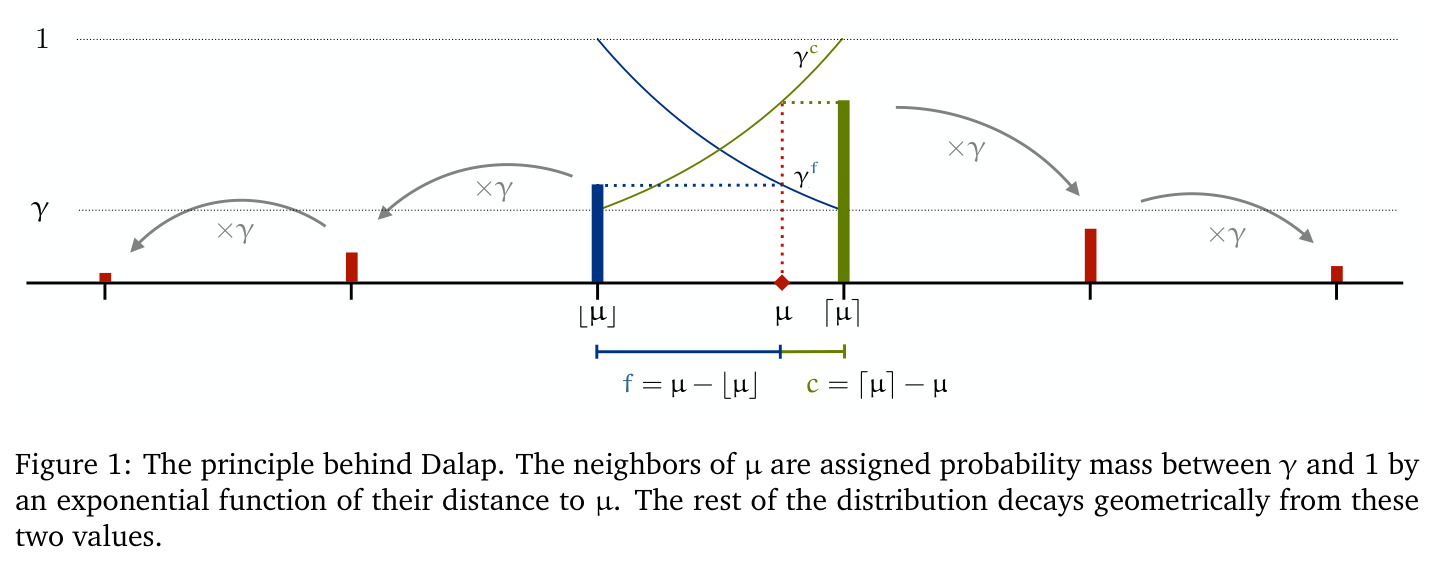
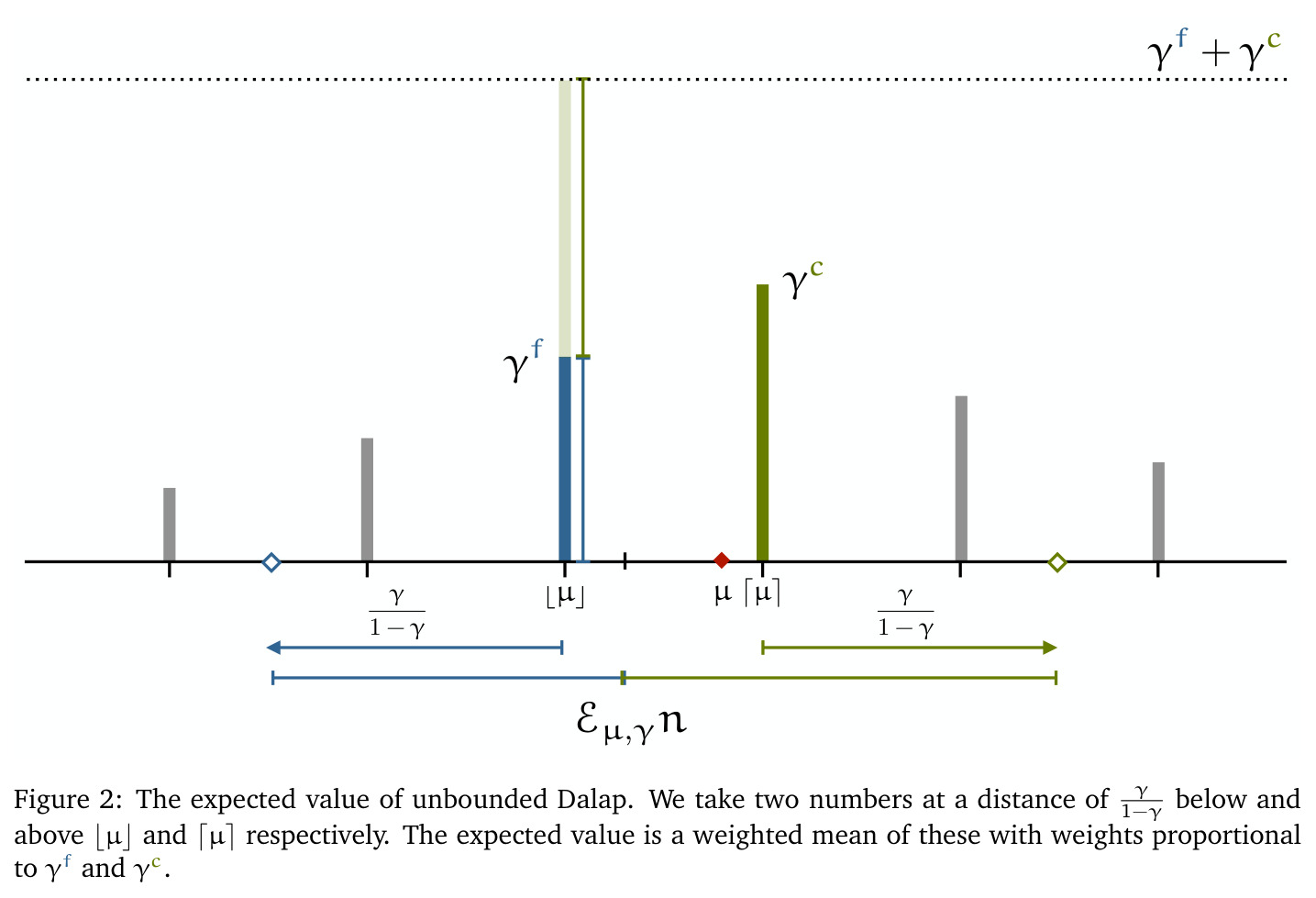
与「离散化连续分布」(先采正态/拉普拉斯再舍入)不同,Dalap 直接构造 $p(n|\mu,\gamma) \propto \gamma^{|n-\mu|}$,$\mu \in \mathbb{R}$ 连续、$\gamma \in (0,1)$ 控制尾部。当 $\mu$ 在两整数之间时,用 $f=\mu-\lfloor\mu\rfloor$、$c=\lceil\mu\rceil-\mu$ 衔接左右尾部,得配分函数 $z = (\gamma^c + \gamma^f)/(1-\gamma)$。创新点:(a) 把 Inusah & Kozubowski (2006) 离散 Laplace 从整数 $\mu$ 拓展为连续 $\mu$,保证梯度;(b) $-\log p(n) = |n-\mu|\log(1/\gamma) + \log z$ 是 $|n-\mu|$ 的线性函数,继承「绝对距离最优」;(c) $\gamma \to 0$ 时方差→0、均值→$r(\mu)$,可表示确定性预测。Bitwise 把每位输出视为独立 Bernoulli,通过符号-数值表示组装成整数分布。
方法步骤详情
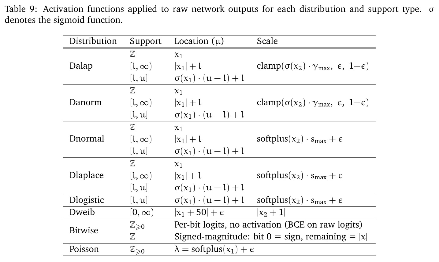
Dalap 迭代流程:(1) 输入经骨干网络得 $h_1, h_2$;(2) Table 9 映射:$\mu$ 用 $h_1$ 或 $\sigma(h_1)(u-l)+l$($[l,u)$),$\gamma$ 用 $\text{clamp}(\sigma(h_2)\cdot\gamma_{\max}, \epsilon, 1-\epsilon)$;(3) 按 $p(n) = (1-\gamma)\gamma^{|n-\mu|}/(\gamma^{\mu-\lfloor\mu\rfloor}+\gamma^{\lceil\mu\rceil-\mu})$ 算概率;(4) 受限情形用 $\gamma^{1+\mu-l}$、$\gamma^{1+u-\mu}$ 修正配分;(5) $\mu$ 越界夹断(Appendix A.5);(6) $-\log p(n)$ 反向传播。Bitwise 把 $n$ 编码为 $k$ 位符号-数值位串,似然 $\prod_i \pi_i^{x_i}(1-\pi_i)^{1-x_i}$,训练按位加权 $2^i$,推理等权。Danorm 配分用 500 项截断近似。
技术新颖性
技术新颖性分四层。第一层是「连续 $\mu$ 的离散类比」——作者显式处理 $\mu \in \mathbb{R}\setminus\mathbb{Z}$ 的情形,引入 $f, c$ 分量并证明配分函数 $z$ 是 $\mu$ 的平滑函数,保证梯度可计算。第二层是「离散类比的正态」——Danorm 把平方指数衰减移植到整数,Proposition 4/5 严格证明均值收敛于 $r(\mu)$、方差趋于 0,这是首次对该分布收敛性质的形式化分析。第三层是 Bitwise 的「概率分布视角」——首次把按位输出显式诠释为 $\mathbb{Z}$ 上的概率分布,并给出 Proposition 6/7/8 的期望、方差公式。第四层是「统一实验对比」——首次把六种候选分布放在表格回归、序列预测、图像生成三大场景下做系统对比,并通过 BPD/RMSE/FID 三指标给出全景观测,这种「方法学上的系统化」本身是稀缺贡献。
实验结果
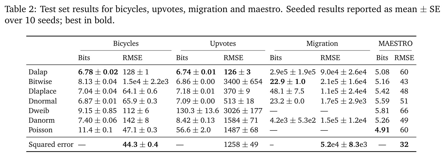
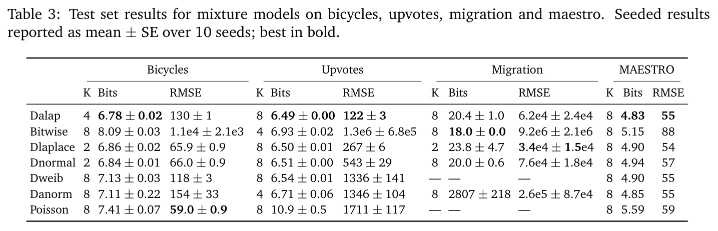
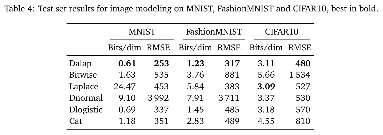
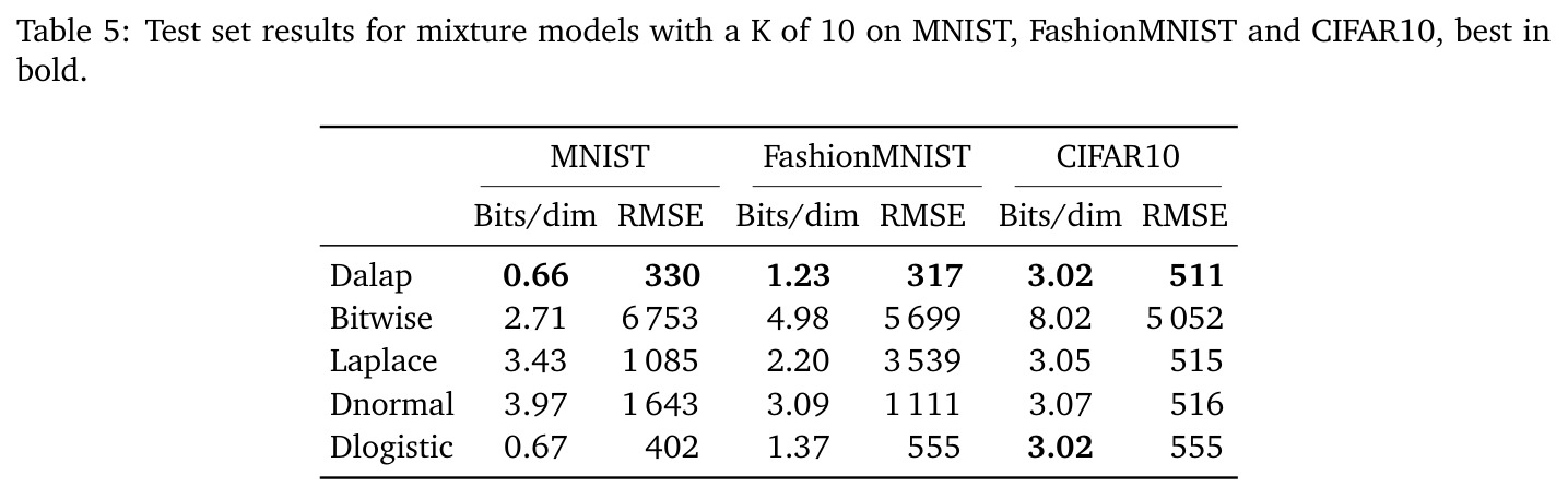
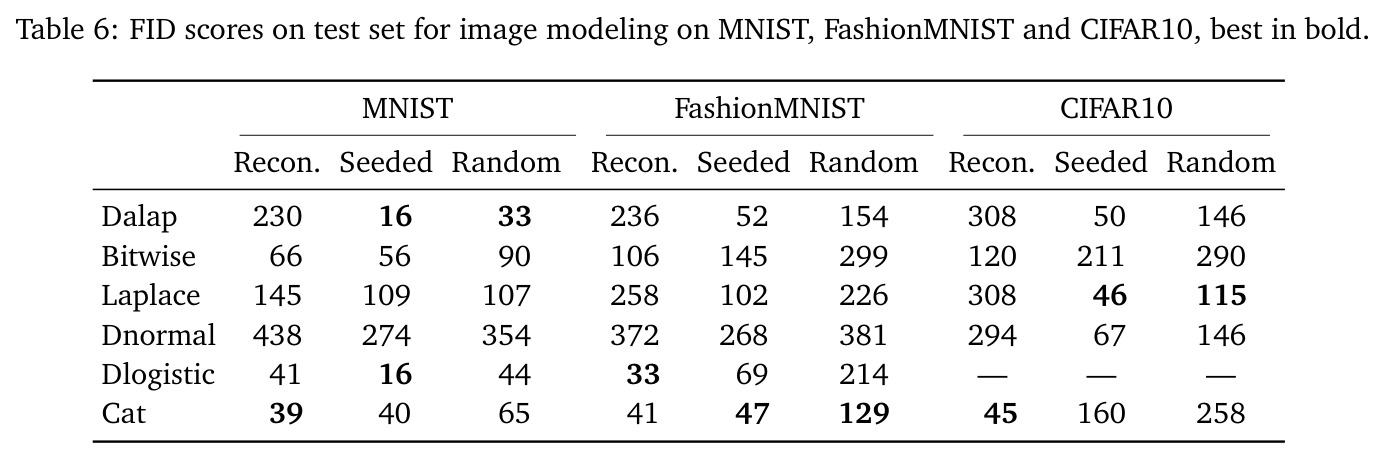
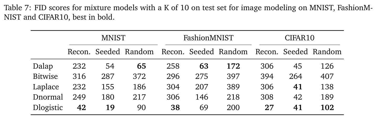
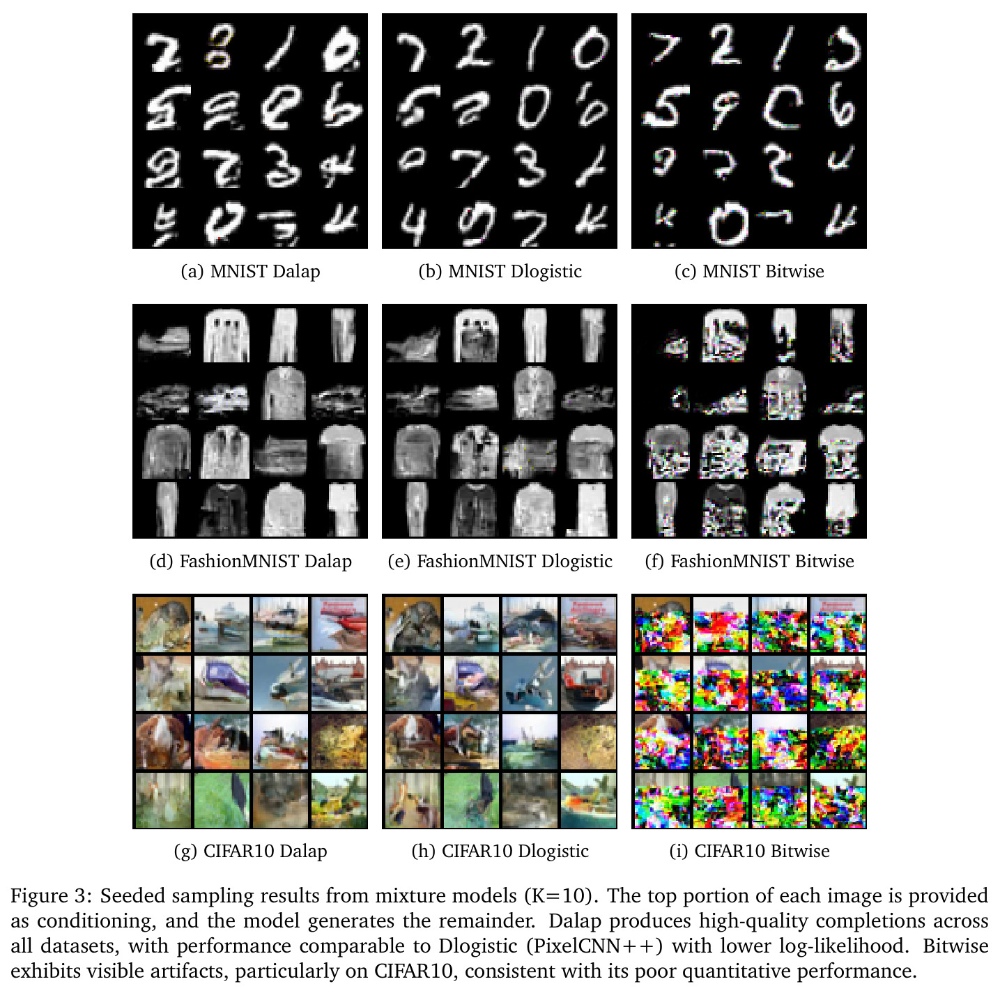
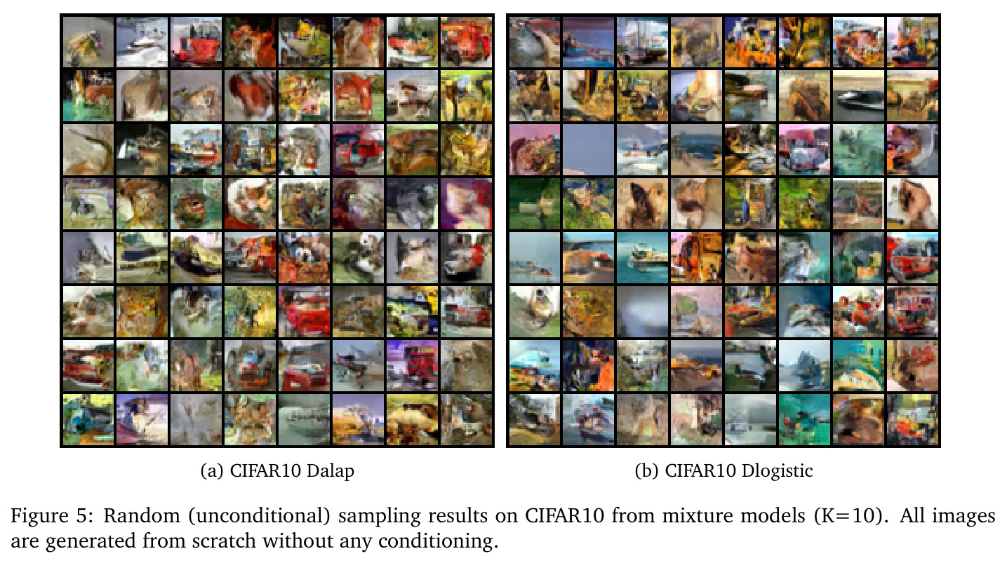
表格回归(Table 2+3):Bicycles 上 Dalap 非混合最低 bits 6.78 ± 0.02,Upvotes 上 Dalap 最优 6.74 ± 0.01;RMSE 上 squared error 在 Bicycles(44.3)比所有离散分布都好(Dalap 128)。Migration 最难(DI=1.85×10⁷),Dalap 非混合 10 seed 中 2 个发散,Bitwise 稳定(22.9 ± 1.0),K=8 混合后 Dalap 追平至 20.4 ± 1.0。MAESTRO 上 Poisson 最优(4.91 bits)。图像生成(Table 4+5):Dalap 在 MNIST(0.61 bpd)、FashionMNIST(1.23)上击败 Dlogistic(0.69、1.45),CIFAR10 上 Dalap 混合 3.0206 bpd 略胜 Dlogistic 的 3.02。Bitwise 在图像失败。生成质量:Dlogistic 在 CIFAR10 重建 FID 26.50 全胜 Dalap 的 306。
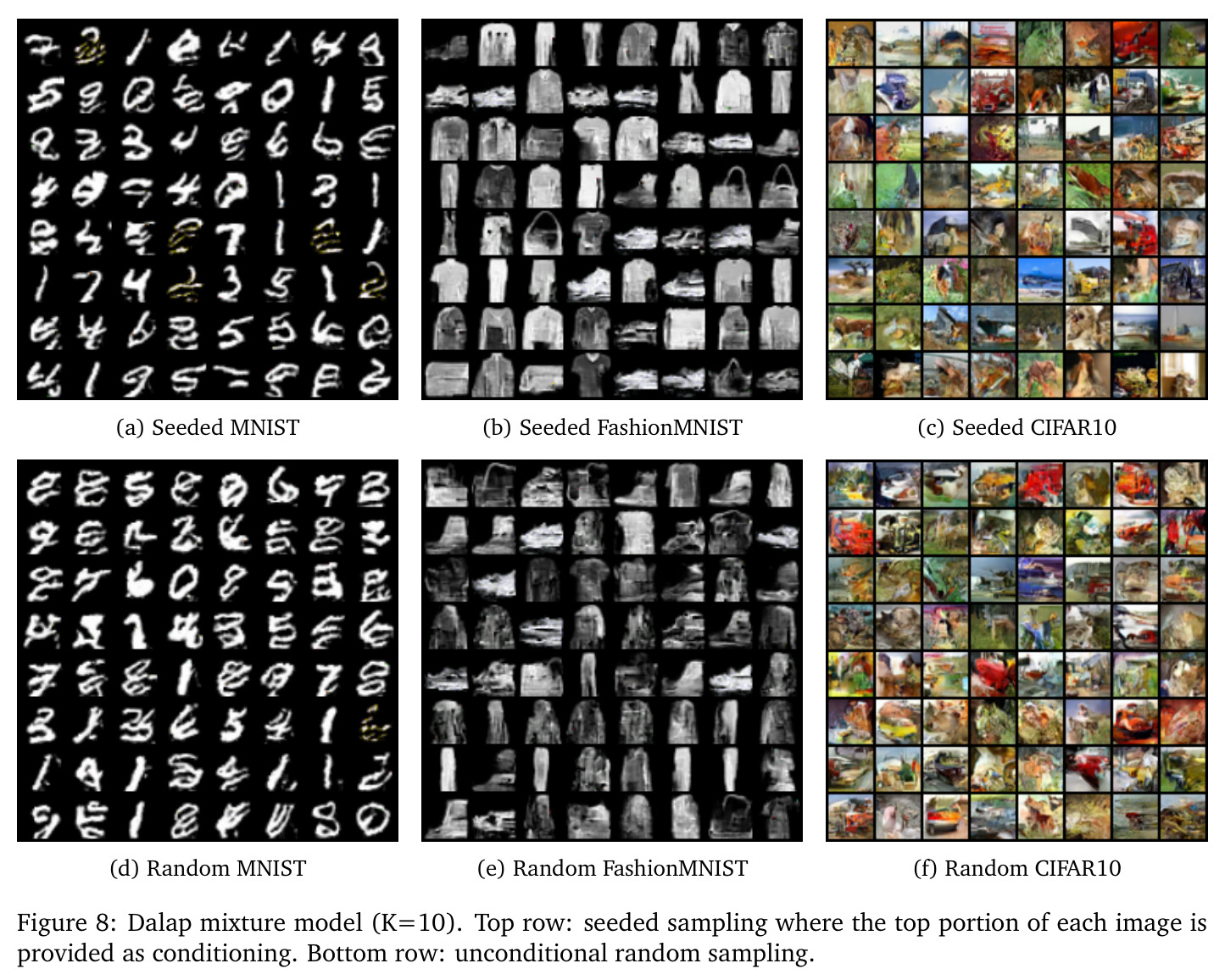
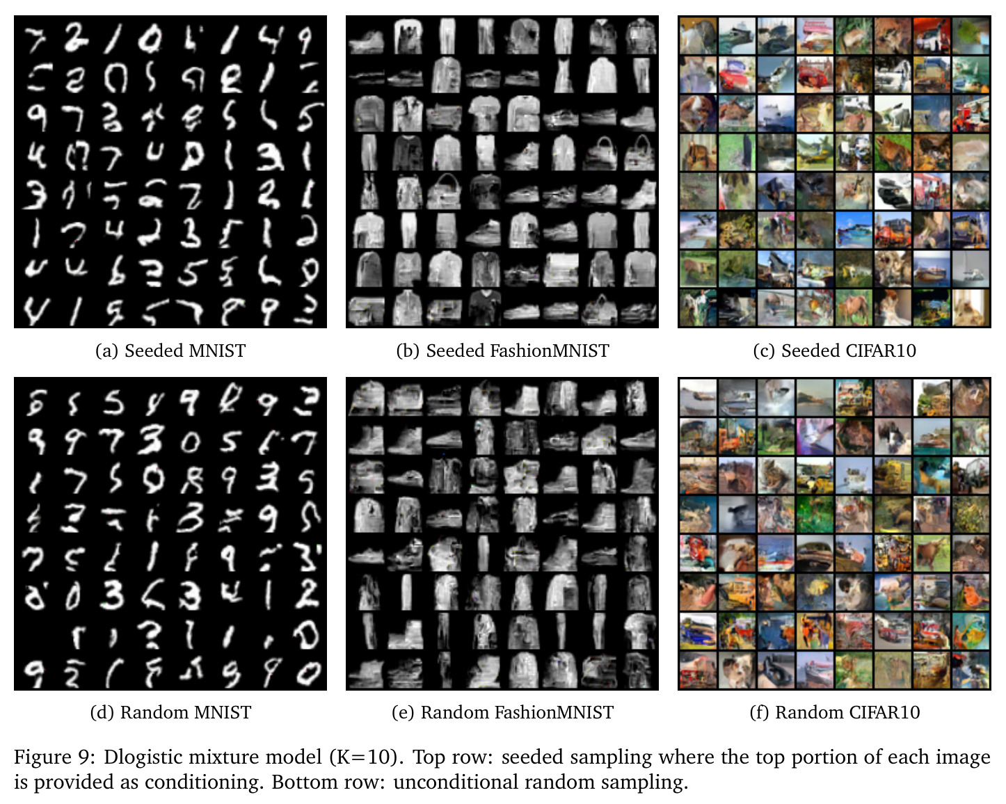
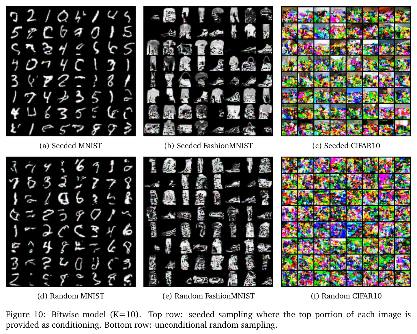
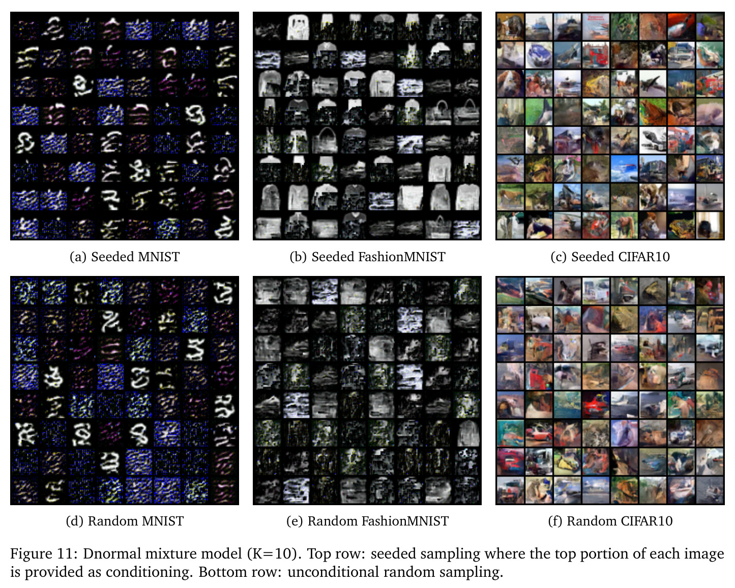
查看结构化数据
| 任务 | 指标 | 本文 | 基线 | 提升 |
|---|---|---|---|---|
| Bicycles 自行车数量预测(表格) | Bits(负对数似然,越低越好) | Dalap 6.78 ± 0.02(非混合) | Dnormal 6.87;Dlaplace 7.04;Poisson 11.4 | 相对最强基线 Dnormal 提升 1.3%;相对 Poisson 提升 40.5% |
| Upvotes 点赞数预测(表格) | Bits | Dalap 6.74 ± 0.01;混合 K=8 时 6.49 | Dnormal 7.09;Poisson 56.6 | 相对 Poisson 提升 88.5%;混合时进一步下降 3.7% |
| Migration 净迁徙预测(表格) | Bits | Dalap 混合 K=8:20.4 ± 1.0;Bitwise 混合 K=8:18.0 ± 0.0 | Dlaplace 混合 K=2:23.8 ± 4.7;Dnormal 混合 K=8:20.0 ± 0.6 | Bitwise 在该数据集胜出,相对 Dalap 提升 11.8%;Dalap 与 Dnormal 接近 |
| MAESTRO MIDI tick 预测(序列) | Bits | Dalap 混合 K=8:4.83 | Poisson 4.91;Bitwise 5.15;Dlogistic 不适用 | 相对 Poisson 提升 1.6%;Poisson 在该数据集最具竞争力 |
| MNIST 像素预测(图像) | Bits per dimension | Dalap 0.61(非混合);0.66(混合 K=10) | Dlogistic 0.69;Dnormal 9.10;Laplace 24.47 | 相对 Dlogistic 提升 11.6%;比 Laplace 提升 97.5% |
| CIFAR10 像素预测(图像) | Bits per dimension | Dalap 混合 K=10:3.0206 | Dlogistic 混合 K=10:3.02;Laplace 混合:3.05 | 相对 Dlogistic 提升约 0.07%;与最强基线持平 |
| MNIST 随机采样 FID(生成质量) | FID(越低越好) | Dalap 混合 K=10:64.75 | Dlogistic 混合 K=10:90;Dnormal 混合 K=10:217 | 相对 Dlogistic 提升 28.1% |
| CIFAR10 重建 FID(图像重建) | FID | Dalap 混合 K=10:306 | Dlogistic 混合 K=10:27 | Dlogistic 在重建任务上大幅领先(FID 约低一个数量级),Dalap 不适合重建 |
局限与改进
作者承认的限制有三:(1) 图像实验受算力限制只跑了 1 个 seed(PixelCNN++ 单次需多 GPU 日),无法给出置信区间;(2) Danorm 在图像生成上需 90GB+ VRAM 计算配分函数,被排除在图像实验外;(3) Dweib 在 Upvotes 数据集上严重发散(130.3 ± 13.6 bits),因 $p(X=x)=\exp(-\beta/\alpha^\beta - (x+1)/\alpha)^\beta$ 的尾部衰减与极端重尾不兼容。独立观察还有几个隐含局限:第一,$\gamma \to 0$ 时 $-\log p$ 爆炸,需 $\epsilon=1e-12$ 截断,实际部署无法做到真正确定性预测;第二,Bitwise 在 Bicycles/Upvotes 上 RMSE 数量级惊人(1.5×10⁴、3400),因位级误差经 $2^i$ 权重放大;第三,Dalap 在 MAESTRO 上赢 Poisson,但当数据不服从时 Poisson 反而更稳定,提示分布族选择是经验性的,没有 universal winner。
独立分析的弱点
从独立视角看有四个弱点。**弱点 1:Dalap 配分函数对 $\mu$ 的依赖**——在 $[l,u]$ 受限下 $z$ 是 $\mu$ 的函数,$\log z$ 项施加非平凡正则化(Appendix A.3 显示它奖励非整数 $\mu$),与 $|n-\mu|\log(1/\gamma)$ 项的张力需精细平衡。改进方向是显式解耦两项或对 $\log z$ 归一化。**弱点 2:Bitwise 训练-评估不一致**——训练按 $2^i$ 加权,评估等权,造成目标不对齐。改进方向是改用期望解码或加入解码后整数误差作为辅助项。**弱点 3:Danorm 算力门槛过高**——90GB VRAM 让单机研究者无法在 PixelCNN 上实验。改进方向是利用 $\gamma^{(n-\mu)^2}$ 在 $\mu$ 上的平移不变性用 FFT 复用配分函数。**弱点 4:缺乏最优性判别准则**——只证渐近性质,无有限 $\gamma$ 下分布族选择规则。改进方向是基于数据矩(DI、kurtosis)做自动分布选择,类似 AutoML 的模型选择。
未来方向
作者明确提出两个未来方向:(1) 把 Dalap 集成进完整的 MIDI 自回归生成模型(不止 tick 预测子任务);(2) 解决 Danorm 在高维场景下的内存爆炸问题,使其能用于图像生成。基于本文结果可延伸的方向:第一,把混合从「K 个独立分布求和」升级为「层级混合」或「注意力加权混合」;第二,把 Dalap 拓展到多维联合整数分布(如 RGB 三通道);第三,探索 Bitwise 的非二进制编码(base-3/base-4)能否减少位数并保持序数结构;第四,把 $\gamma$ 取值与数据特征(DI)建立解析对应关系让分布族选择自动化;第五,从信息论视角研究 Dalap 相对最优编码的 regret bound;第六,把框架应用到 NLP 离散 token 生成(若 token 表存在序数结构可压缩参数)。
复现评估
复现性整体良好但有门槛。代码——第 3 页脚注提供 https://github.com/pbloem/contin 开源仓库。数据——7 个数据集全公开:Bicycles 来自 Fanaee-T (2013),Upvotes 来自 Naseer (2020) 比赛,Migration 来自 World Bank Group (2024),MAESTRO V3 来自 Hawthorne et al. (2019),MNIST/FashionMNIST/CIFAR10 来自 torchvision。算力——表格 + MAESTRO 单 GPU 数小时可完成;PixelCNN++ 图像每模型需多 GPU 日,作者无法做多 seed;Danorm 图像需 90GB VRAM。难度——论文给了详尽公式推导、数值稳定性细节(Appendix A.5)、激活函数表(Table 9),但 Dalap 的 $f, c$ 处理、Bitwise 加权、Danorm 近似都易出 bug。风险——PixelCNN++ 只跑 1 seed 且未做 K 网格搜索,复现最优 bits 有方差。
论文图表
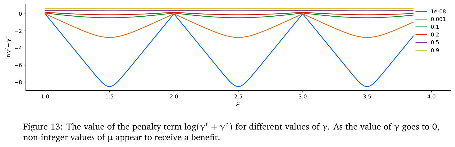
三维曲面图:x 轴是 $\gamma \in (0, 1)$,y 轴是 $f \in [0, 1]$,z 轴是 $\log(\gamma^f + \gamma^{1-f})$。曲面在 $f=0.5$ 处($\mu$ 位于两个整数中点)出现「塌陷」,即当 $\gamma \to 0$ 时该项数值变为负且很大,似乎奖励非整数 $\mu$。
可视化揭示 Dalap 损失中 $\log z$ 项的反直觉行为,是 Appendix A.3 详细数学论证的入口——读者必须先看到这张图才能理解为何作者要专门写一段论证解释「看似奖励非整数 $\mu$,实际上仍要付出距离代价」。